Feasibility of coupling a thermal/optical carbon analyzer to a quadrupole mass spectrometer for enhanced PM_2.5 speciation

Figures & data

Figure 1. Schematic of the TOA-QMS system for PM_2.5 organic carbon and inorganic species measurement.

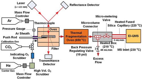
Figure 2. (a) Thermogram from burning of a birch log collected on a quartz-fiber filter comparing the IMPROVE_A temperature protocol with the simplified protocol used with the TOA-QMS; (b) TOA-QMS spectrum obtained for the 580°C portion from m/z 10 to 250, which constitutes most of the evolved gases. Major features are noted at m/z 27, 39, 44, 91, and 115.

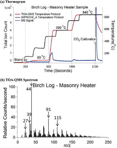
Figure 3. CO₂ ionization efficiency (error bars of ±1 standard deviation derived from replicate analyses are smaller than the size of the dots).

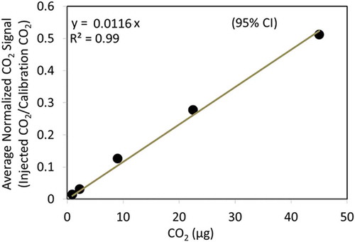
Figure 4. Calibration curves for (a) ammonium, (b) nitrate, (c) sulfate, and (d) organic carbon using oxalic acid (C₂H₂O₄). Error bars indicates ±1 standard deviation derived from replicates. The y-axis shows the corresponding summed species m/z signals from the TOA-QMS normalized using the CO₂ calibration peak m/z signal and divided by the filter punch area in cm². The x-axis values were obtained from quantification by IC and TOA analysis of portions of the filter standards. Linear regression curves are forced through zero.

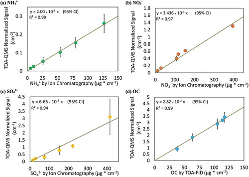
Figure 5. TOA-QMS and EI-AMS spectra for (a) NH₄NO₃, with the most abundant peaks at m/z 14, 15, 16, 17, 18, 30, and 46; (b) (NH₄)₂SO₄, with the most abundant peaks observed at m/z 14, 15, 16, 17, 18, 32, 48, 64, 80, 81, and 98; (c) C₂H₂O₄ with the most abundant peaks for TOA-QMS at m/z 29, 44, 45, and 46, and for EI-AMS at m/z 16, 17, 27, 28, 43, 44, and 45; and (d) CO₂ with the most abundant peak at m/z 44.

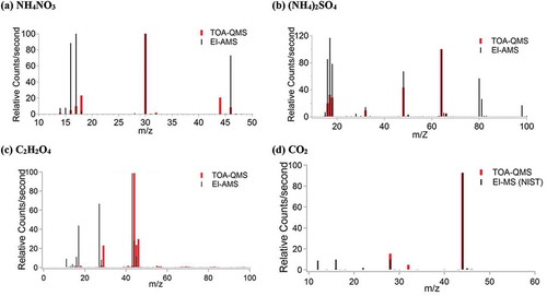
Table 1. Fragmentation patterns and interference corrections for ammonium, nitrate, and sulfate.

m/z	Ion	Interference ion	Calculation of interference ion	Corrected m/z signal for species
	Ammonium
14	N^+	N^+ (from NO3)	0.0178 × m/z 30 (NO^+→N^+) 0.17818 × m/z 46 (NO2^+→N^+)	Signal at m/z 14, interference fragment
15	NH^+	Organic	Small interference from organic	0.0802 × m/z 16
16	NH2^+	Organic	Small interference from organic	Signal at m/z 16
17	NH3^+	OH^+ (from H2O)	0.2122 × m/z 18	Signal at m/z 17, interference fragment
	Nitrate
14	N^+	Organic	Small interference from organic	0.0178 × signal at m/z 30 + 0.17818 × signal at m/z 46
30	NO^+	Organic at m/z 29	0.022 × m/z 29 (assumed organic)	Signal at m/z 30, interference fragment
31	NO^+	Organic	Small interference from organic	0.00405 × signal at m/z 30
32	NO^+	Organic	Small interference from organic	0.002 × signal at m/z 30
44	N2O^+	Organic at m/z 44	Small interference from organic	2 × signal at m/z 46 + 0.2 × signal at m/z 30
46	NO2^+	Organic	Small interference from organic	Signal at m/z 46
47	NO2^+	Organic	Small interference from organic	0.00443 × signal at m/z 46
48	NO2^+	Organic	Small interference from organic	0.004 × signal at m/z 46
Sulfate
18	Fragment of SO3	H2O	Small interference from organic	0.49 × signal at m/z 48 + 0.268 × signal at m/z 64
48	SO^+	NO2^+	Nitrate at m/z 48 m/z 62 (assumed organic)	Signal at m/z 48, interference fragment
64	SO2^+	Organic	0.5 × m/z 50 (assumed organic) 0.5 × m/z 78 (assumed organic)	Signal at m/z 64, interference fragment

Figure 6. Spectrum processing flow diagram showing how interferences are removed from overlapping m/z signals.

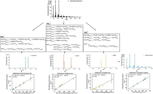
Figure 7. TOA-QMS concentrations vs. (a) NH₄⁺ by IC, (b) NO₃⁻. by IC, (c) SO₄^2- by IC, and (d) OC by TOA for samples collected in Fresno, CA, and Baltimore, MD. Samples from the western United States, such as those from Fresno, CA, are rich in NO₃⁻, while samples from the eastern United States, such as those from Baltimore, are rich in SO₄^2-.

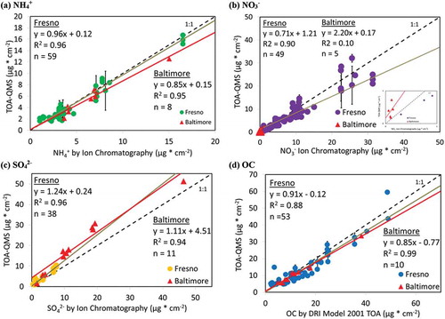
Figure 8. Average (colored bars) and standard deviations (black lines) of major chemical components in 58 Fresno, CA, samples measured by TOA-QMS, IC, and TOA. Elemental carbon (EC), soil, and salt concentrations determined from TOA, x-ray fluorescence (XRF), and atomic absorption spectrometry (AA), but not by TOA-QMS, are included for completeness. The NO₃⁻ offset is apparent, but the low SO₄^2- averages are in reasonable agreement, as are the NH₄⁺ and OC averages. The soil is calculated using the following formula: Soil = 2.2Al + 2.49Si + 1.63Ca +1.94Ti + 2.42Fe (Malm et al. 1994).

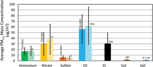
Figure 9. TOA-QMS mass concentration for (a) NO₃⁻ by IC adjusted with a factor of 1.36 plotted vs. IC mass concentration and (b) SO₄^2- by IC adjusted with a factor of 0.80.

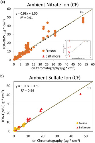
Figure 10. OC and ion contributions to PM_2.5 determined by TOA-QMS at the Fresno Supersite from 12/15/200 to 02/03/2001. Five samples were collected for each day (i.e., 0000–0500, 0500–1000, 1000–1300, 1300–1600, and 1600–2400 local standard time [LST]). Highest concentrations of OC and NO₃⁻ were observed during the late afternoon to night time period (1600–2400 LST).

Malm, W.C., J.F. Sisler, D. Huffman, R.A. Eldred, and T.A. Cahill. 1994. Spatial and seasonal trends in particle concentration and optical extinction in the United States. J. Geophys. Res. 99:1347–70. doi:10.1029/93JD02916.

 Web of Science ®Google Scholar