Revisiting the Veterans Cohort Mortality Study: New results and synthesis

Figures & data

Table 1. Veterans Administration hypertension clinics used in the analysis.

Allen Park	MI (Detroit)
Birmingham	AL
Buffalo	NY
Chicago	IL
Cleveland	OH
Dallas	TX
Dayton	OH
East Orange	NJ (Newark)
Houston	TX
Indianapolis	IN
Iowa City	IA
Jackson	MS
Los Angeles	CA
Memphis	TN
Miami	FL
Milwaukee	WI
Minneapolis	MN
New Orleans	LA
Oklahoma City	OK
Omaha	NE
Philadelphia	PA
Pittsburgh	PA
Richmond	VA
Salt Lake City	UT
San Francisco	CA
Seattle	WA
St. Louis	MO
Topeka	KS
Tucson	AZ
Washington	DC
West Haven	CT (New Haven)

Figure 1. Trends in veterans’ and U.S. male mortality rates.

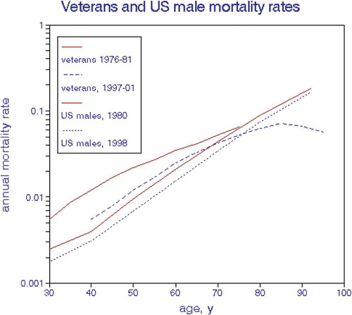
Table 2. Mean values of air quality and traffic variables.

	Exposure periods
Variable	≤1975	1976–1981	1982–1988	1989–1996	1997–2001
A. From EPA ambient monitors
TSP (μg/m^3)	96	74	59
PM10 (μg/m^3)				39
PM2.5 (μg/m^3)				14	13
PM10 –2.5 (μg/m^3)				16
SO4^2− (μg/m^3)	11	8.6			3.6
Non-SO4^2− PM2.5 (μg/m^3)		6.2
NO2 (ppb)	30	27	24	21	16
Peak O3 (ppb)	76	92	63	45	19
Peak CO (ppm)	11	(7.6)*	(3.4)*	2.4	1.6
B. From the Inhalable Particulate Network (IPN)
PM2.5 (μg/m^3)		24	22
PM15 (μg/m^3)		45	43
PM10–2.5 (μg/m^3)		21	21
SO4^2− (μg/m^3)		7.5	(6.7)*
C. ln(traffic density (10^6 veh-km/km^2)	1.89	1.90	1.91	1.92
D. From the EPA Speciated Trends Network (STN)
Elemental C (μg/m^3)				0.62
NO3^− (μg/m^3)					1.84
Ni (ng/m^3)					1.73
V (ng/m^3)					1.9
PM2.5 (μg/m^3)					14
PM10 (μg/m^3)					31
SO4^2− (μg/m^3)				3.6
Peak SO2 (Ppb)				16
Peak O3 (Ppb)				19
Peak CO (Ppm)					1.6
Mean NO2 (Ppb)				20
Mean O3 (Ppb)					52
14 other PM2.5 constituents that were not significant
E. From nationwide dispersion modeling
SO2 (ppb)					4.3
NOx (ppb)					19.5
Elemental C (μg/m^3)					0.82
SO4^2− (μg/m^3)					3.9*
F. From the EPA Hazardous Pollutant Emissions Inventory (ng/m^3)
Benzene					1528
Formaldehyde					1155
Diesel particulates					1810
Nickel					2.09
Polycyclic organics					6.4
Local mercury					0.57
Lead					141
Arsenic					0.15
Chlorine					19.1
Hydrochloric acid					168
Polypropylene					0.18
Manganese					3.08

Notes. Means of modeled air quality are subject weighted. Peak values are 95th percentiles. All others are arithmetic means. Bold indicates P < 0.05 in at least one regression with concurrent exposure and mortality.

*Parentheses indicate negative effect.

Table 3. Mean concentrations by data source.

	EPA monitors
Pollutant	STN data	IPN data^#	AER modeling	HAP estimate
SO4^2− (μg/m^3)	8.6*	3.6	6.7	3.9
EC (μg/m^3)	0.62			0.82
Diesel PM (μg/m^3)		1.81
PM2.5 (μg/m^3)	13	14	22
PM10,15 (μg/m^3)	31		43
NO2 (ppb)	16	20	20 (NOx)

Notes. *Includes filter artifacts.

^#1979–1983.

Table 4. Relative mortality risks for counties with ambient air quality monitors.

	Exposure		Mortality period
Pollutant	Period	Mean	1976–1981	1982–1988	1989–1996	1997–2001	1976+
TSP	<1975	96	0.971	0.993	0.881		0.983
	1976–1981	74	1.005	0.960	0.861		1.031
	1982–1988	59		1.052	0.991		1.057
PM10	1989–1996	39			1.101		1.165
	1997–2001	30				1.121
Average (SD)			0.988 (0.024)	1.002 (0.47)	0.959 (0.11)		1.059 (0.077)
SO4^2−	<1975	11.2	1.025	1.00			0.999
	1976–1981	10.9	1.019	1.047	1.061		1.055
	2002*	3.9				1.036	0.936
Average (SD)			1.022 (0.004)	1.012 (0.016)			0.997 (0.060)
PM2.5	1979–1981	24	0.906	0.829	0.751		0.829
	1982–1984	22		0.916	0.857		0.887
	1989–1996	14.3			1.118		1.005
	2002	14.3				1.026	1.026
Average (SD)				0.873	0.989 (0.19)		0.965 (0.13)
NO2	<1975	30	1.062	1.057	1.062		0.990
	1976–1981	27	1.094	1.069	1.074		1.040
	1982–1988	24		1.032	1.035		0.995
	1989–1996	21			1.052		1.002
	1997–2001	20				1.120	1.084
NOx	2002*	31					1.182
Average (SD)			1.078 (0.021)	1.053 (0.018)	1.056 (0.016)		1.049 (0.074)
Peak O3	<1975	76	0.971	0.989	0.987		0.960
^#	1976–1981	92	1.056	1.059	0.995		1.053
	1982–1988	63		1.110	1.048		1.082
	1989–1996	45			1.106		1.113
	1997–2001	19				1.050	1.013
Average (SD)			1.013 (0.042)	1.051 (0.049)	1.034 (0.048)		1.044 (0.054)
ln(VKTA)	1985*	1.90					1.022
	1997*	1.90	1.051	1.054	1.052	1.055	1.060
Average (SD)							1.041 (0.027)

Notes. Bold indicates P < 0.05.

*Risks based on modeled exposures.

^#Based on mean − minimum concentrations.

Table 5. Summary of lag effects.

Pollutant	Mean RR	Lag coefficient (standard error)	Regression standard error
All particulates	1.009	−0.0046 (0.0021)	0.088
Peak O3	1.067	−0.0042 (0.0012)	0.045
Mean NO2	1.052	—	0.038

Figure 2. Effects of current smoking status on mortality risk, based on proportional hazards regression coefficients by age group and time period.

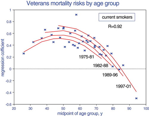
Figure 3. Effects of current smoking status on mortality risk, based on proportional hazards regression coefficients by age group and time period, showing average years of birth.

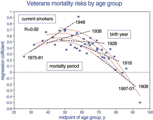
Figure 4. Effects of current smoking status on mortality risk, based on proportional hazards regression coefficients by age group, time period, and birth year.

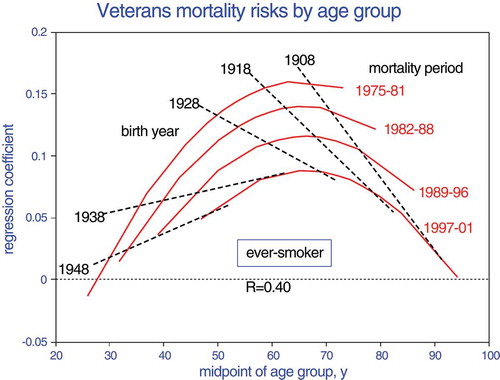
Figure 5. Effect of living in poverty on mortality risk, based on proportional hazards regression coefficients by age group.

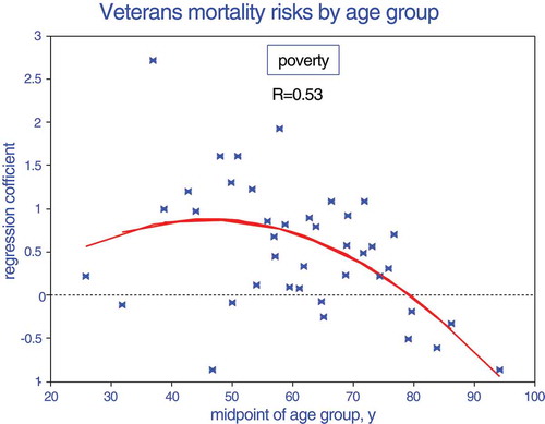
Figure 6. Effect of county space heating degree-days, based on proportional hazards regression coefficients by age group and time period.

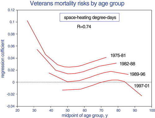
Figure 7. Average mean effects of traffic density by age at recruitment, less minimum and maximum estimates.

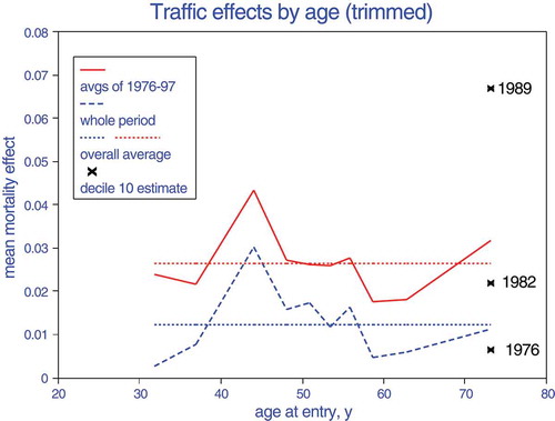
Figure 8. Average mean effects of benzene by age at recruitment, less minimum and maximum estimates.

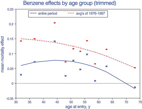
Figure 9. Effect of exposure to nitrogen oxides on proportional hazards mortality regression coefficients.

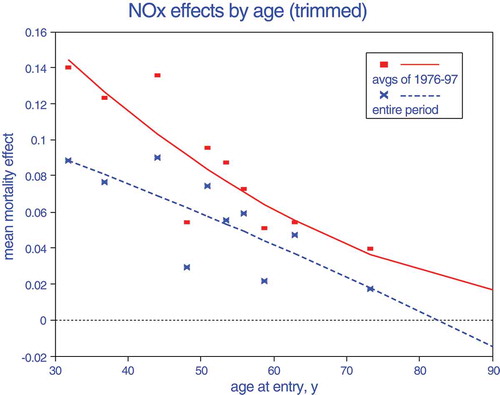
Table 6. Mean pollutant values by age decile.

Decile	Age	AER NOx (μg/m^3)	Benzene (ng/m^3)	ln(VKTA)
1	25.9 (2.8)	20.6 (12.8)	1565 (582)	1.957 (1.57)
2	36.9 (3.3)	21.1 (13.8)	1568 (608)	1.996 (1.66)
3	44.1 (1.35)	20.1 (12.8)	1516 (606)	1.871 (1.71)
4	48.1 (0.95)	19.6 (13.9)	1489 (609)	1.817 (1.77)
5	50.9 (0.75)	19.4 (13.9)	1483 (607)	1.798 (1.72)
6	53.4 (0.69)	19.6 (14.1)	1486 (617)	1.785 (1.75)
7	55.8 (0.72)	19.6 (14.3)	1486 (617)	1.765 (1.75)
8	58.7 (0.97)	19.6 (14.4)	1474 (621)	1.747 (1.75)
9	62.9 (1.5)	19.3 (14.3)	1480 (622)	1.777 (1.74)
10	73.2 (5.9)	18.8 (14.0)	1480 (615)	1.732 (1.74)

Notes. Standard deviations in parentheses.

Table 7. Summary of mean risks (ln[RR]) by follow-up period.

Follow-up period	Smoking	ln(VKTA)	AER NOx	Benzene
1976–2001	0.451 (0.048)	0.0124 (0.0026)	0.056 (0.0085)	0.054 (0.014)
1976–1981	0.388 (0.048)	0.0203 (0.0120)	0.113 (0.0276)	0.095 (0.055)
1982–1988	0.468 (0.040)	0.0281 (0.0056)	0.118 (0.0258)	0.134 (0.028)
1989–1996	0.465 (0.063)	0.0283 (0.0091)	0.071 (0.0165)	0.132 (0.032)
1997–2001	0.302 (0.126)	0.0291 (0.0116)	0.039 (0.0217)	0.107 (0.049)
Average over periods	0.406	0.0264	0.0853	0.117
(Standard error of mean)	0.039	0.0021	0.0190	0.010
Relative risks	1.50	1.027	1.089	1.124

Notes. Bold indicates P < 0.05.

Table 8. Summary of relationships with mortality.

Variable	Correlation (R^2)	RR*
Current smoking status (Figures 2,3)	0.85	2.11
Degree-days (Figure 6)	0.55	1.11
Height (per inch)	0.38	1.01
Traffic density (Figure 7)	0.36	1.05
Poverty (Figure 5)	0.28	2.23
Mean benzene (Figure 8)	0.27	1.16
Mean nox (Figure 9)	0.23	1.16
Ever smoked (Figure 4)	0.16	1.18
Race (minimum RR)	0.14	(0.84)
Education (minimum RR)	0.08	(0.95)

Notes. Bold indicates P < 0.05.

*For positive (adverse) relationships, the maximum RR is listed. For negative relationships, the minimum is listed.

Figure 10. Example of potential public health importance of age-related air pollution risks based on vital statistics for U.S. males in 2000. Life-years lost are expressed in thousands; premature deaths, in hundreds.

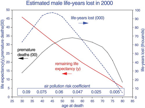
Table 9. Summary of findings.

Issue	Response
Are contextual variables required?	Yes, they improve overall model fit.
How was the WUSTL model validated?	Our estimated risks from smoking compare well with exogenous estimates. Air pollution risk estimates are consistent across subset analyses.
Which monitored pollutants are most important?	Maximum risks from single-pollutant regressions are similar for all pollutants but lower for CO, SO4^2−, and PM2. 5.
Are nonmonitored pollutants important?	Yes, risks associated with traffic density and most HAPs are statistically significant and often stronger than for criteria pollutants. Traffic density acts as a surrogate for other factors.
Do exposures in locations monitored by EPA represent the whole country?	No, nationwide analyses show that most of the risks are limited to routinely monitored areas.
Do risk estimates differ by region?	Yes, traffic-related pollutants tend to prevail, suggesting that the other pollutants are less important.
Are multipollutant regressions useful?	Yes, traffic-related pollutants tend to prevail, suggesting that the other pollutants are less important.
Are estimated risks coincident with exposures?	Yes, greater responses are seen with coincident exposures.
How important is cohort follow-up time?	Traditional cohort studies do not distinguish between cohort aging and temporal changes in covariates, which pose differing implications.
Do mortality risks vary substantially by age?	Yes, pollution risk coefficients tend to decrease with age. Pollution-associated deaths tend to peak around age 60.
What can be learned from subset analyses?	Trends and geographic gradients can be defined more precisely. Sums of subset effects may exceed estimates based on the whole cohort because of changes in covariates.

Table 10. Coherence of relative risk estimates (as elasticities) based on various data sets and follow-up periods for all ages.

	Traffic pollutants		Particulates		Peak ozone
NO2 (1)*	1.049	TSP (1)	1.057	Table 3, 1976–1981	1.056
NO2 (2)	1.090	PM10 (1)	1.165	Table 3, 1982–1988	1.110
		PM10 (2)	1.121	Table 3, 1989–1996	1.106
NOx (4)	1.182	PM2.5 (1)	1.005	Table 3, 1997–2001	1.050
		PM2.5 (6)	0.887	STN counties (2)	1.051
EC (2)	1.140	PM2.5 (2)	1.092
EC (4)	1.146	SO4^2− (1)	1.055
Diesel PM (5)	1.051	SO4^2− (2)	1.036
Traffic density(3)	1.060	SO4^2− (4)	0.936
Mean (SEM)	1.102 (1.05–1.15)		1.039 (0.98–1.10)		1.075 (1.04–1.11)

Notes. Bold indicates P < 0.05.

*Data sources: (1) routine EPA monitoring; (2) the EPA STN database; (3) traffic count data;

(4) nationwide dispersion modeling; (5) emission rates of hazardous pollutants; (6) the Inhalable Particulate Network (IPN).

Table 11. Statistical significance and correlations (in parentheses) in 2-pollutant models.

	ln(VKTA)	EC	peak O3
ln(VKTA)		Y (0.36)	Y (0.14)
EC	Z (0.36)		Z (−0.27)
Ni	Z (0.31)	X (0.39)	Y (−0.12)
Polycyclic organics	Z (0.26)
NOx	Z (0.27)
benzene	Z (0.68)
V	X (0.10)	0 (0.59)	Y (−0.17)
NO2	X (0.46)
peak CO	X (−0.12)
NO3^−	X (0.53)	0 (0.12)
SO4^2−	X (0.16)		0 (0.43)
PM2.5	X (0.63)		0 (0.22)
Diesel PM	Y (0.54)
Formaldehyde	Y (0.75)

Notes. X = pollutant in the column heading is significant; Y = pollutant in the row heading is significant; Z = both pollutants are significant (pairwise correlation); 0 = neither pollutant is significant. Blank entries were not tested.