Novel cross-flow electrostatic precipitator: Numerical and experimental study

Figures & data

Figure 1. Cross-flow schematic (Ali et al. 2016)

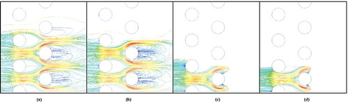
Figure 2. Mutual coupling of physical phenomena in electrostatic precipitators (ESP’s)

Figure 3. Computational domain for cross-flow electrostatic precipitator (TP, LP = 10 mm; CE diameter = 5 mm; DE diameter = 1 mm)

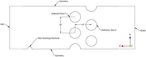
Figure 4. Meshed grid for the cross-flow ESP configuration

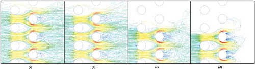
Table 1. Hydrodynamic and electrical boundary conditions for the cross-flow model

Boundaries	Hydrodynamic B.C.	Electrical B.C.
Inlet	$u_x=u_{\mathrm{\infty }};u_y=0$
Outlet	Pressure Outlet
Domain Wall Boundaries	Symmetric: $\mathrm{\partial }{u}_y/\mathrm{\partial }y=0$	$\mathrm{\partial }q/\mathrm{\partial }y=0and\mathrm{\partial }V/\mathrm{\partial }y=0$
Collector Wall	No-Slip Wall: $\overrightarrow{u}=0$	$V=0and\text{break}\left(\mathrm{\partial }q/\mathrm{\partial }x=0;\mathrm{\partial }q/\mathrm{\partial }y=0\right)$
Discharge Wire	No-Slip Wall: $\overrightarrow{u}=0$	$V=V_{\mathrm{\infty }}$
Particle	No-Slip Wall: $\overrightarrow{u}=0$	$V=0\left(Initial\right)$

Table 2. Computation parameter setting for the modeling of flow domain in cross-flow ESP

Parameters	Settings
Simulation Type	2D, Steady Double Precision, Pressure Based, and Implicit
Temporal Discretization	2^nd Order
Turbulence Model	Realizable k-ε
Turbulent Wall Treatment	Enhanced Wall Treatment
Pressure	Standard
Pressure-Velocity Coupling	SIMPLE
Momentum	2^nd Order Upwind
Turbulent Kinetic Energy	2^nd Order Upwind
Turbulent Dissipation Rate	2^nd Order Upwind

Table 3. Model constants

Model Constants
Free-space permittivity $\left({\epsilon }_o\right)$	$8.85\times {10}^{-12}\mathrm{C}/\mathrm{V}.\mathrm{m}$
Density of air $\left({\rho }_{air}\right)$	$1.225\mathrm{k}\mathrm{g}/{\mathrm{m}}^3$
Dynamic viscosity of air $\left({\mu }_{air}\right)$	$1.8\times {10}^{-5}\mathrm{k}\mathrm{g}/\mathrm{m}.\mathrm{s}$
Relative permittivity of fly-ash $\left({\epsilon }_r\right)$	3.0
Density of fly-ash $\left({\rho }_{fly-ash}\right)$	$860\mathrm{k}\mathrm{g}/{\mathrm{m}}^3$
Peek’s electric field $\left(E_{Peek}\right)$	$3.33\times {10}^7\mathrm{V}/\mathrm{m}$
Positive ions mobility $\left({b_i}^{+}\right)$	$1.8\times 10^{-4}{\mathrm{m}}^2/\mathrm{V}\cdot \mathrm{s}$
Ion mass $\left(m_i\right)$	1.30 × 10 − 24 kg

Figure 5. Subdomain of interest and result locations

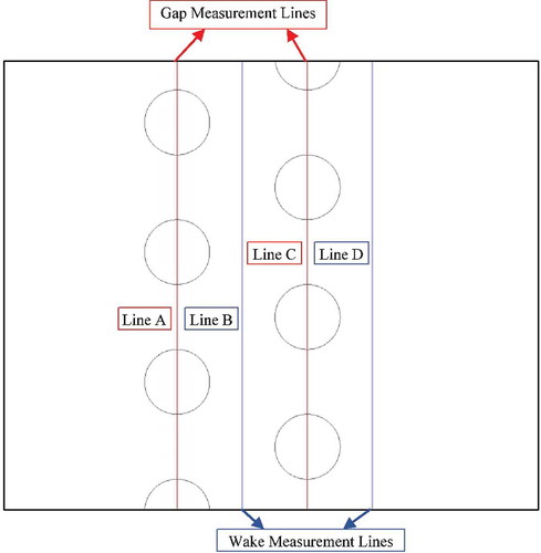
Figure 6. Comparison of velocity field distributions (as well as velocity vector plots) for flow across cross-flow cells (a) 0.25 m/s; (b) 1 m/s

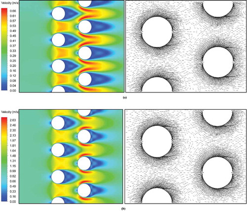
Figure 7. nondimensional transverse flow (simulation) profiles across interstitial gaps for normalized mean velocity (a) Gap velocity profile (simulation) results across Row 1(b) Gap velocity profile (simulation) results across Row 2 (c) Wake velocity profile (simulation) results across Row 1 (d) Wake velocity profile (simulation) results across Row 2

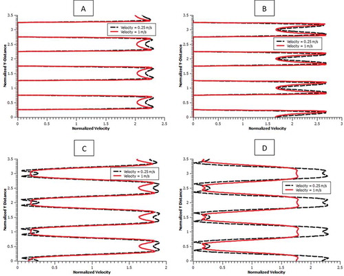
Figure 8. nondimensional transverse flow (simulation) profiles across interstitial gaps for normalized turbulence intensity (a) Gap turbulence profile (simulation) results across Row 1(b) Gap turbulence profile (simulation) results across Row 2 (c) Wake turbulence profile (simulation) results across Row 1 (d) Wake turbulence profile (simulation) results across Row 2

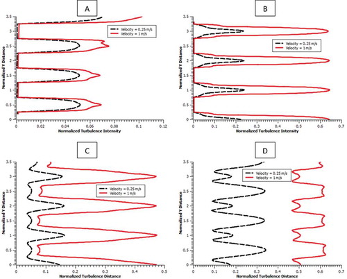
Figure 9. Electric field distribution in the collector zone of the cross-flow ESP for an applied voltage of 70 kV (a) X-component of local electric field distribution; (b) Y-component of local electric field distribution;(c) Magnitude of the local electric field distribution; (d) Global field distribution within the domain; (e) Charge density distribution at the electrode

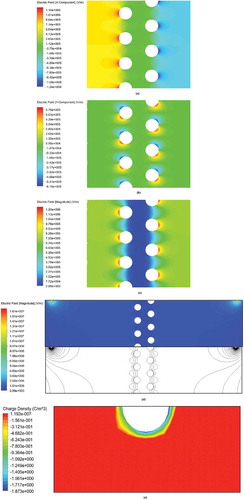
Figure 10. Global particle trajectory in a cross-flow ESP with an applied voltage of 70 kV (a) 0.25 m/s; (b) 1 m/s

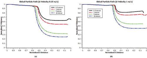
Figure 11. Local particle collection for inlet velocity of 0.25 m/s in a cross-flow ESP with an applied voltage of 70 kV (a) 0.5 μm; (b) 1 μm; (c) 5 μm; (d) 10 μm

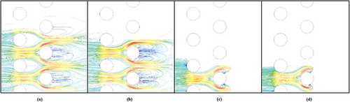
Figure 12. Local particle collection for inlet velocity of 1 m/s in a cross-flow ESP with an applied voltage of 70 kV (a) 0.5 μm; (b) 1 μm; (c) 5 μm; (d) 10 μm

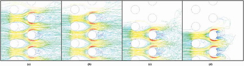
Table 4. Collection efficiency w.r.t particle size and inlet velocity

	Inlet velocity = 0.25 m/s	Inlet velocity = 1 m/s
0.5 $\text{mum}$	57.4%	25.14%
1 $\text{mum}$	86%	34.57%
5 $\text{mum}$	100%	80.57%
10 $\text{mum}$	100%	100%

Figure 13. Cross-flow ESP experimental system

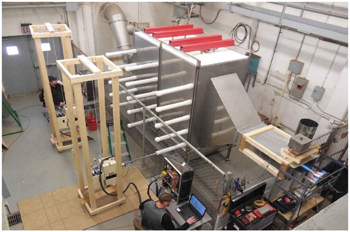
Figure 14. Cross-flow ESP experimental schematic (top view)

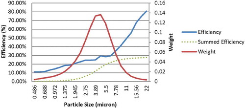
Figure 15. Particle size distribution used in the experimental study

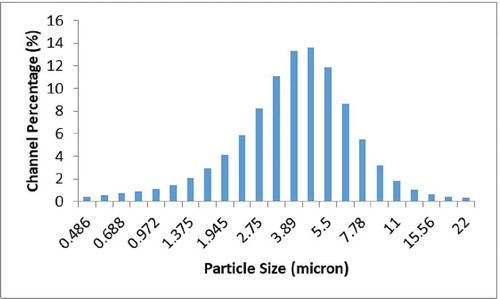
Figure 16. Channel efficiency of simulation model for particle size distribution used in the experiment

Ali, M., H. Pasic, K. Alam, S. Tiji, N. Mannella, T. Silva, and T. Liu. 2016. Experimental study of cross-flow wet electrostatic precipitator. J. Air Waste Manage. Assoc. 66 (12):1237–44. doi:10.1080/10962247.2016.1209258.

 PubMed Web of Science ®Google Scholar