
Figures & data
Figure 1. Locations of Texas Commission of Environmental Quality (TCEQ) monitors (blue) and Houston Regional Monitoring (HRM) network sites (magenta) in Houston, TX. Red area outlines are locations of regulated entities. Green lines are county boundaries and blue lines are major roadways. Arrows represent hourly averaged wind speed and direction.
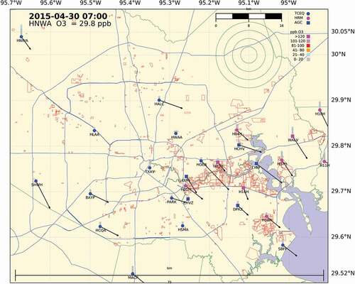
Figure 2. The average 1-hour wind vectors for 2000–2015 at 27 monitors for (left) exceedance days and (right) non-exceedance days. The data is also separated by (top) March to July and (bottom) August to October. An exceedance day is determined if the daily maximum 8-hour ozone concentration is greater to or equal than 70 ppb. Colors indicate the time of day, and each dot is the wind vector tail.
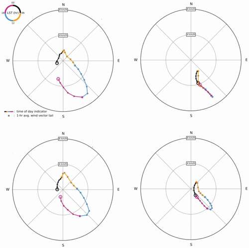
Table 1. Exceedance statistics for observations during 2000–2015 for 21 TCEQ regulatory monitors, and 6 HRM monitors. An exceedance is defined as having a 1-hour O3 measurement equal or greater than 100 ppb.
Figure 3. For the HO3H monitor for 2015 the number of compass quadrants (1Q-4Q) traversed by the wind direction during a 24-hour period. Also shown are the number of days with no exceedances (0X), a one-hour exceedance (1X) ≥ 100 ppb, 8-hour average exceedance (8X) ≥ 70 ppb or has a one-hour and eight-hour exceedance (9X).
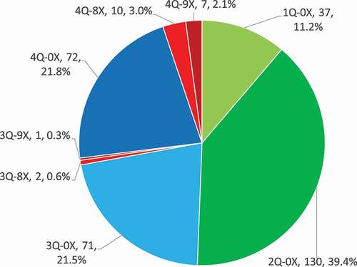
Figure 4. For the Houston HO3H monitor, during 0–6 LST, the starting wind direction (color) and the morning transport distance versus 8-hour (8-H) averaged ozone concentrations for April 1 – October 1 for (Top) 2012 and (Bottom) 2015.
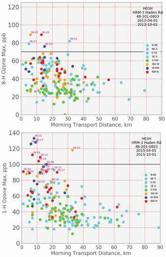
Figure 5. For the HO3H monitor the midnight wind direction, the number of compass quadrants the wind direction traversed over 24 hours for Apr 01-Oct 01 of (left) 2012 and (right) 2015. Also shown are the number of days for each quadrant with no exceedances (0X), 8-hour average exceedance (8X), or has a one-hour and eight-hour exceedance (9X).
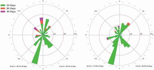
Figure 6. For the BAYP monitor the displacement, ozone concentration, wind speed and direction for the (top) May 2012 and (bottom) May 16–20, 2012. Black stair-stepped line is the 1-Hour average ozone, and the red horizontal bar is the computed highest 8-Hour average ozone for the day. The blue stepped line is the 1-Hour resultant wind speed arriving at site where the blue text on the right-side y-axis label provides the wind speed. The multicolored lines and dots at top of chart are the hourly kilometer displacement of flowsto and away from the site, and are centered at noon at the site. The colored segments are each 6 hours long, small gray circles mark each hour, and the kilometer scale of displacement is shown in the upper left of plot with a color code for each 6-hour segment. The magenta digit and letter “q,” are the number of wind quadrants occurring in each displacement plot. The black numbers next to 1 h ozone is the annual rank of the 1 h ozone maximum value (only shown for days with ranks 1–60) and the red numbers next to the 8 h ozone is the same for the 8 h ozone maximum value.
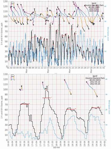
Figure 7. The (A) San Antonio Camp Bullis, (B) El Paso UTEP, and (C) HGB HNWA monitors for 2015 with the number of compass quadrants (1Q-4Q) traversed by the wind direction during a 24-hour period. Also shown are the percentage and number of days for each quadrant. Also shown are whether there are no exceedances (0X), 8-hour average exceedance (8X), or a one-hour and eight-hour exceedance (9X).
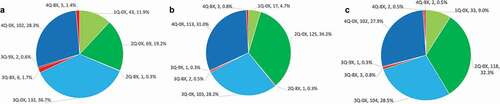
Figure 8. Composites of light-wind trajectories at 500 m from radar wind profilers operating in Texas in May–October 2005 and 2006. Each trajectory lasts 24 hours and is assumed to terminate at the profiler site at 1800 LST (0000 UTC). Colors indicate time of trajectory segments, and numbers indicate total number of wind days included in the composite for each profiler. To be included, the day’s resultant wind speed must be less than 3 m/s.
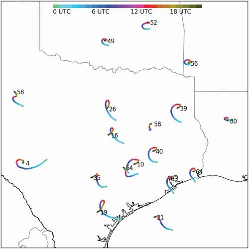
Figure 9. One-day modeled mixed-layer wind trajectories with varying background wind strengths. Winds are modeled with a straight coastline oriented similar to Houston, TX. Numbers along the trajectories indicate hours after trajectory starting point: 0 = 18:00 LST; 6 = Midnight LST; 12 = 0600 LST the next day; 18 = Noon LST the next day; 24 = 18:00 LST the next day.
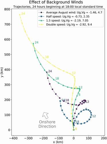
Figure 10. Modeled mixed-layer wind hodographs with varying background wind strengths. Colors indicate time of day as in . Hodograph is drawn with wind vector tails (originating) along the circles and wind vector heads (terminating) at 0,0. Negative velocities correspond to winds from the south and/or west. All hodographs are circular, but only the average and half-speed hodographs encircle the origin and thus produce winds that perform a complete rotation.
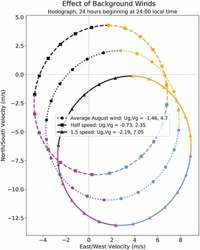
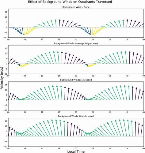
Figure 11. The effect of background winds on the number of quadrants that modeled winds traverse in a day. Arrows represent wind vectors at each hour of the day, colors indicate individual compass quadrants. The top subplot is with no background winds. The subplots below it shows modeled winds using the climatological average for mean boundary-layer winds over Houston in August (u = −1.46 m/s, v = 4.70 m/s) at 100%, 150%, and 200% of average speed.
Supplemental Material
Download Zip (5.5 MB)Data availability statement
The data that support the findings of this study are openly available in UNC Dataverse at 10.15139/S3/BP5B95, 10.15139/S3/7DNRJP and 10.15139/S3/YAVDSI.