PM_2.5 in Carlsbad Caverns National Park: Composition, sources, and visibility impacts

Figures & data

Figure 1. Active oil and natural gas wells near Carlsbad Caverns National Park (CAVE) (HIFLD, 2019). The color bar gives the number of active O/G wells in the given grid cell. The grid cell resolution is 0.1 degree by 0.1 degree. Cells with 500 or more active wells are shown with the same color. National Park boundaries are shown in green. Larger cities in the surrounding area are marked with black dots and labeled. The monitoring site, in CAVE is shown as a yellow star. Coal-fired power plants in the region are shown as yellow plus signs (U.S. EIA, 2022).

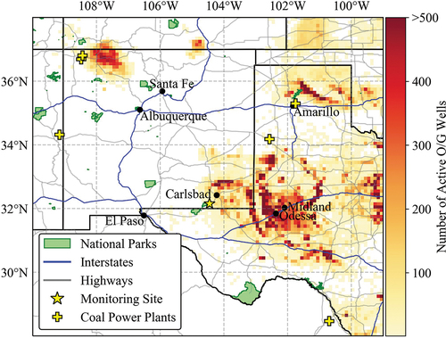
Table 1. Measurements made during the CarCavAQS study are listed with their respective time-resolutions and measured species. Only instruments used in this work are listed. Abbreviations used for the measured species: sodium (Na⁺), ammonium (NH₄⁺), calcium (Ca²⁺), potassium (K⁺), magnesium (Mg²⁺), chloride (Cl⁻), nitrite (NO₂⁻), nitrate (NO₃⁻), sulfate (SO₄^2-), organic carbon (OC), black carbon (BC), elemental carbon (EC), ammonia (NH₃), nitric acid (HNO₃), sulfur dioxide (SO₂).

Sampling Technique	Measured Species	Time Resolution	Limit of Detection
Aerosol
URG filter pack	PM2.5 ions (Cl^−, NO2^−, NO3^−, SO4^2-, Na^+, NH4^+, K^+, Ca^2+, Mg^2+) Carbohydrates (levoglucosan (C6H10O5))	24-hour	0.01 µg m^−3 for PM2.5 ions, 0.01 ng m^−3 for levoglucosan
Aethalometer	PM2.5 BC	2-minute	0.01 µg m^−3
TEOM	PM2.5 mass	6-minute	0.1 µg m^−3
PILS-IC	PM2.5 ions (Cl^−, NO2^−, NO3^−, SO4^2-, Na^+, NH4^+, K^+, Ca^2+, Mg^2+)	13-minute integrated sample every 30 minutes	0.08 µg m^−3 for Mg^2+, 0.01 µg m^−3 for all other ions
PILS-TOC	PM2.5 WSOC	2-minute	0.01 µg m^−3
IMPROVE module A	PM2.5 mass and elemental composition	24-hour, every 3^rd day	0.3 µg m^−3 for PM2.5, 0.01–0.06 µg m^−3 for elemental analysis
IMPROVE module B	PM2.5 ions (Cl^−, NO2^−, NO3^−, SO4^2-)	24-hour, every 3^rd day	0.001–0.01 µg m^−3
IMPROVE module C	PM2.5 OC and EC	24-hour, every 3^rd day	0.1 µg m^−3 for OC and 0.02 µg m^−3 for EC
Gases
URG denuders	Inorganic gases (NH3, HNO3, SO2)	24-hour	0.01 µg m^−3
Picarro Cavity Ringdown Spectrometer	CH4	15-second	7 ppbv
Eco Physics NO Analyzer	NO, NO2, NOy	1-minute	20 pptv

Figure 2. Time series of major PM_2.5 species and CH₄ measured at the monitoring site. (a.) BC measured by the Aethalometer at 880 nm, WSOC measured by the PILS-TOC, and PM_2.5 measured by the TEOM. Note that there is a gap in the PILS-IC and PILS-TOC data at the beginning of the study period associated with a power outage. The BC and WSOC are plotted at a time-resolution of 2-minutes. TEOM total PM_2.5 is plotted at an hourly resolution. (b.) The five PILS-IC species with the largest contributions to total PM_2.5 are plotted at 30-minute time-resolution. (c.) CH₄ measured by the Picarro at 15-second time-resolution. Shaded regions represent case study transport dates.

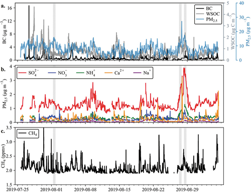
Figure 3. URG annular denuder/filter pack sampling shows the particle/gas phase partitioning of (a.) NH₃/NH₄⁺, (b.) HNO₃/ NO₃⁻, and (c.) SO₂/ SO₄^2-. Particle species are shown in Orange, and gas species are shown in blue. There is one day of missing data, 2019–08-04, due to a denuder extraction error.

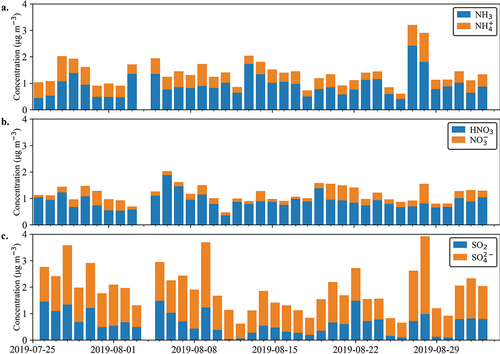
Figure 4. PILS-IC species (a.) NH₄⁺ and SO₄^2-, and (b.) NO₃⁻ and Na⁺ are shown as nano equivalents m⁻³. Shaded regions represent case study transport dates.

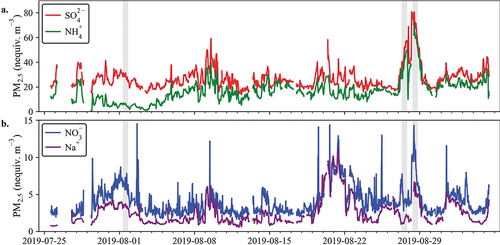
Figure 5. The ratio of cation to anion species measured by the PILS-IC is plotted in equiv. m⁻³. The dotted gray line shows a ratio of unity. The radius of the Orange point size changes proportionally with Ca²⁺ concentration. Shaded regions represent case study transport dates.

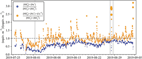
Figure 6. 48-hour HYSPLIT Back Trajectories are shown for three different transport patterns during the study. The bottom panel shows back trajectory altitudes above ground level. The dates were selected based on aerosol composition. For each date 12 daytime back trajectories of 48-hour duration are plotted.

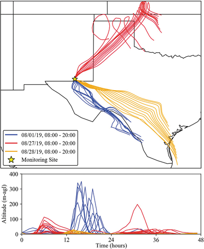
Figure 7. (a.) IMPROVE mass closure is plotted in the upper panel. Reconstructed PM_2.5 mass is shown as the sum of OM, fine soil, (NH₄)₂SO₄, NH₄NO₃, and EC. The IMPROVE measured PM_2.5 mass is also shown by the black dots. (b.) The contribution to light extinction from each species plotted in (a.) as calculated using the second IMPROVE algorithm for light extinction. Site specific Rayleigh Scattering (10 Mm⁻¹) and NO₂ light extinction are also included. NO₂ (g) light extinction is calculated using the second IMPROVE algorithm and a daily mean of the measured NO_2.

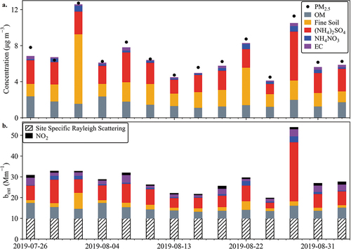
Figure 8. The second IMPROVE equation was applied to higher time resolution composition data sets (PILS-IC, PILS-TOC, and Aethalometer BC) to estimate hourly light extinction values. These values include the Rayleigh background contribution as well as extinction from NO₂. Fractional light extinction contributions, excluding Rayleigh background, from different species are shown for three data points (shown as blue triangles) as examples. Extinction peaks highlighting maximum contributions are represented by points a and c (30 July 2019 09:00 MST and 28 August 2019 12:00 MST). Point b represents a low light extinction period on 18 August 2019 12:00 MST.

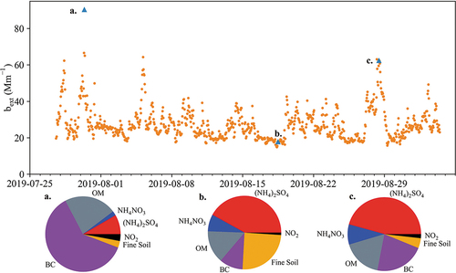
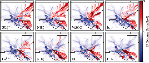
Figure 9. Incremental probability distributions are plotted for 7 species measured directly during the field campaign: SO₄^2-, NH₄⁺, WSOC, Ca²⁺, NO₃⁻, BC, and CH₄ and 1 calculated value: particle light extinction (b_ext). The IPs are based on 24-hr back trajectories and are distance normalized. This is done by multiplying each grid cell value by the distance from the origin site, shown as a black dot. The grid cell resolution is 0.25 degrees square.

Homeland Infastructure Foundation-Level Data (HIFLD). 2019. Oil and natural gas wells. Accessed February 26, 2021. https://gii.dhs.gov/HIFLD.

 Google Scholar

United States Energy Information Administration (EIA). 2022. U.S. Energy mapping system. Accessed March 21, 2022. https://www.eia.gov/state/maps.php.

 Google Scholar

Data availability statement

The data that support the findings of this study are available from the corresponding author, Jeffrey L. Collett, upon reasonable request. https://doi.org/10.25675/10217/235481.