Experimental study of a full-scale hexagonal wet electrostatic precipitator for collection of black carbon and particulate matter generated by a marine diesel engine

Figures & data

Figure 1. Schematic of the experimental setup. Three measurement points are marked with red spots and three gas measurement points are marked with black spots. During the experiments the temperature, T, pressure, P, and gas flow volume, F, were measured.

The electrode used during the experiment is shown in the southeast corner.

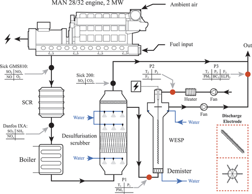
Table 1. Stokes particle diameter intervals and geometric mean Stokes particle diameters.

Impactor stage No. [−]	Stokes diam. range [μm]	Geom. Mean stokes diam. [μm]
1	0.005–0.020	0.01
2	0.020–0.039	0.03
3	0.039–0.068	0.05
4	0.068–0.117	0.09
5	0.117–0.203	0.15
6	0.203–0.302	0.25
7	0.302–0.493	0.39
8	0.493–0.769	0.62
9	0.769–1.302	1.00
10	1.302–1.956	1.60
11	1.956–3.280	2.53
12	3.280–8.171	5.18

Figure 2. Description of the data processing steps for BC, ELPI, and PM.

Figure 3. Illustration of the cumulative probability for ELPI data when the WESP was turned on and off. Five comparison points, marked with a circle and a dashed line, are illustrated where removal efficiency and standard deviation are calculated.

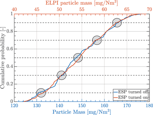
Figure 4. Illustration of normalized current, I_t/I_ref, as a function of time, t, where a spark can be seen in the gray/blue area.

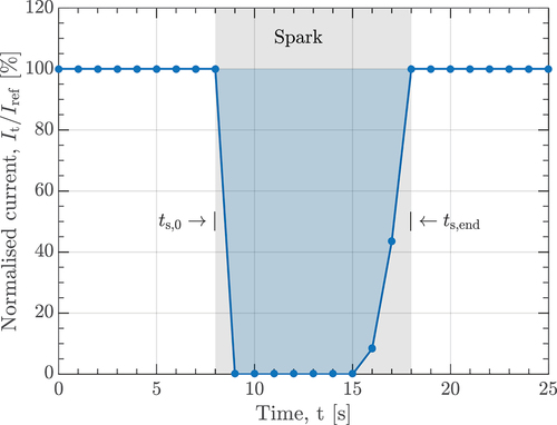
Figure 5. Effect of different discharge electrode lengths as a function of current density, J, and voltage, V.

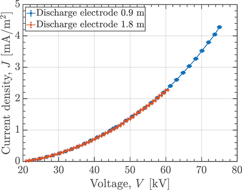
Figure 6. Particle diameter, d_st,p, mass distribution of the gas input for the WESP and their standard deviation.

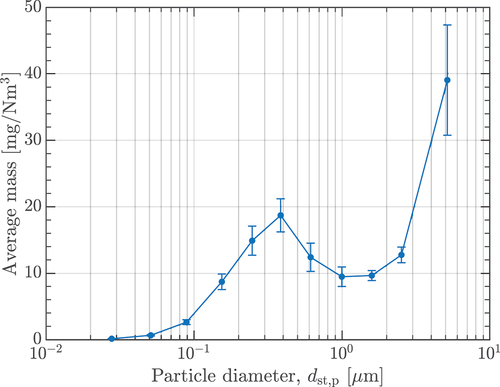
Figure 7. Trapping efficiencies at different particle residence times, t_pr, for particle diameters between 0.02–1.30 µm, 1.30–8.17 µm, the overall range 0.02–8.17 µm, with their percentage of the total mass, m_t, and depicted with standard deviations.

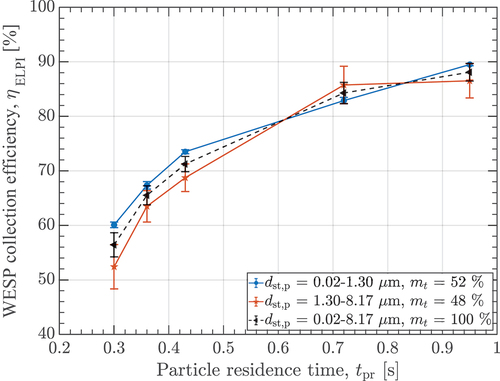
Figure 8. Removal efficiencies for different mean stokes diameters, d_st,p at various particle residence times, t_pr.

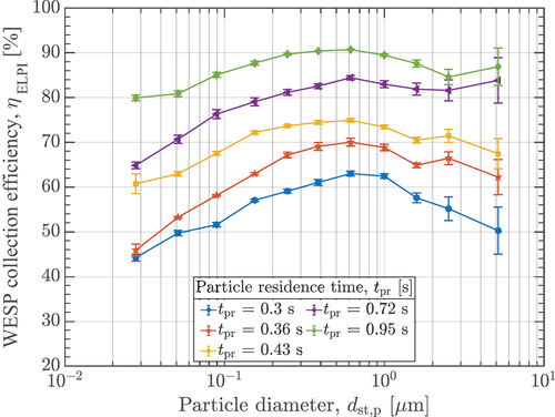
Figure 9. WESP mass trapping efficiency, measured with ELPI, for different electrical energy densities with a constant particle residence time, t_pr, of 0.36 s for (a) and 0.72 s for (b).

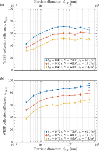
Figure 10. Trapping efficiency of PM (a), BC (b), and ELPI (c) as a function of electric energy density, ρ_e, times the particle residence time, t_pr.

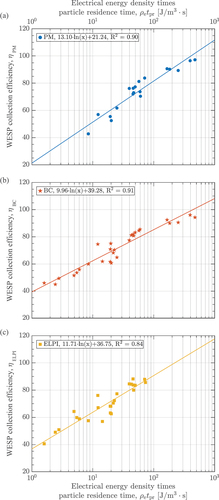
Figure 11. Comparison between PM and BC collection efficiencies, η.

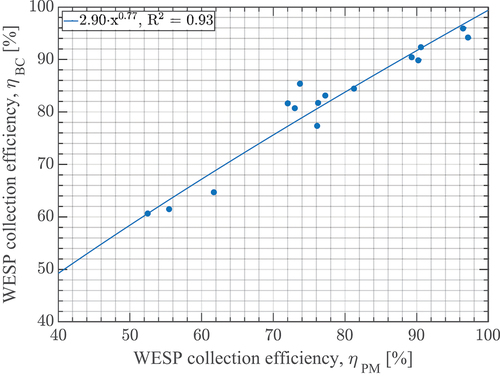
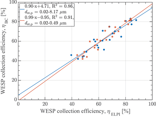
Figure 12. Comparison between ELPI and BC collection efficiencies, η, scatter plot with ELPI data from 0.02–8.17 µm and from 0.02–0.49 µm.

Data availability statement

Raw data were generated at Alfa Lavals test center, Aalborg. Derived data supporting the findings of this study are available from the corresponding author NHH on request.