
Figures & data
Figure 1. Antioch Dunes National Wildlife refuge (green) and a gypsum processing facility (orange) along the San Joaquin River near the Sacramento-San Joaquin River Delta, California.
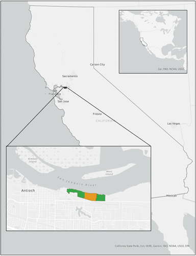
Figure 2. Endangered species protected at the Antioch Dunes National Wildlife refuge. Images publicly available from the U.S. Fish and Wildlife Service (https://www.fws.gov/species/).
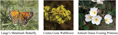
Figure 3. The passive sampler deployed on the Sardis unit with the gypsum facility in the background. The image is facing west-southwest. The gypsum plant is approximately 400 m from this sampler.
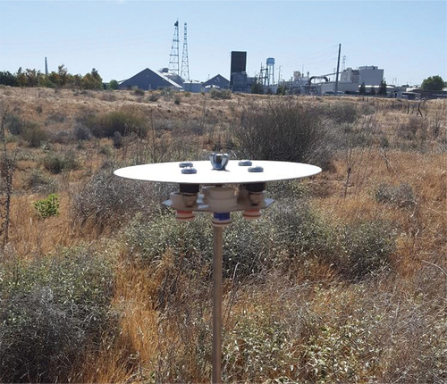
Table 1. Summary of sample collection deployments.
Figure 4. Sampling sites and locations of interest in the Antioch Dunes area. The predominant wind direction is shown along the waterway. The two wildlife refuge parcels are outlined in yellow. The gypsum plant between the two parcels is outlined in red. Site locations are indicated by blue circles. Stolen samplers have a black dot. The site location indicated with a white circle on the Stamm unit is two nearby sampler locations at different elevations.
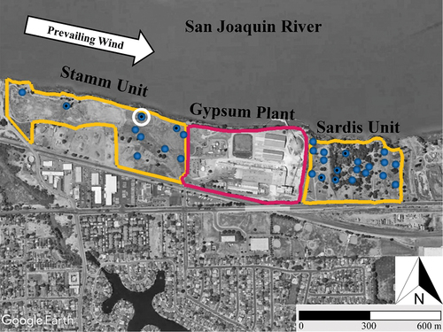
Figure 5. Wind roses for each sampling period. The direction of the paddles is the direction of wind origin. The distance of the paddle from the plot center for each plot represents the frequency of observations at that direction, in percent. The fill colors show the observed wind speed for each fraction of each paddle. The sum of all paddles in each plot equals 100%.
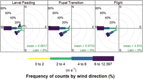
Table 2. Summary of wind speed and direction during each sampling period.
Figure 6. Replicate precision results from reanalysis of ten collected samples. The horizontal dashed line shows the 20% limit used in laboratory QC screening protocols.
Table 3. Summary of measured parameters and detection levels. The Sardis and Stamm columns indicate the mean and one standard deviation of the abundance (ppm) for each parcel.
Figure 7. The variability of collocated sample sets is shown using violin distributions. The ordinal plane represents the measured values divided by the lowest value observed for each parameter and sample set. The violin shape is the vertically oriented frequency distribution observed for each of these ratios. The ordering of the abscissa is from the lowest to highest measured loading for each sample set; hence, the first position consists entirely of measured/Minimum=1. The horizontal dotted line indicates a ratio of 1, indicating no measurable difference, while the horizontal dashes line indicates a ratio of 2, for reference.
Figure 8. The variability of collocated sample sets by parameter using boxplots. Most parameters lie within the 20–50% range except for Na, Cl, Cu, and Ba. Sulfur shows a different profile between the upwind and downwind monitoring locations while other elements are much more similar.
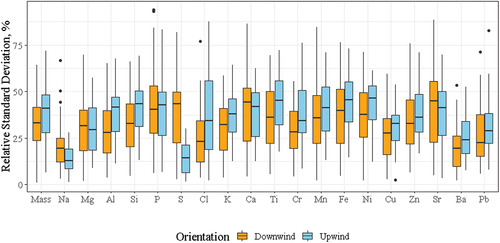
Figure 9. Spatial distribution of median loadings from four selected elements. The median values were taken from the entire study period. The top two maps, sodium and potassium, were selected to represent natural background elements in aerosols. Sodium is predominantly related to sea salt while potassium comes primarily from minerals and wood smoke. The bottom two maps, calcium and sulfur, show a pronounced difference between upwind and downwind locations. These elements are related to gypsum.
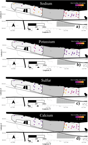
Figure 10. Ratios of downwind/upwind loadings by parameter shown with columns for each sampling period. The dashed line indicates a ratio of 1, indicating no difference. The downwind/upwind ratio is generally conserved across sampling periods. The three gypsum elements, S, Ca, and Sr are clearly distinct.
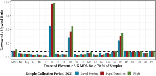
Figure 11. Enrichment of downwind elemental loadings with respect to upwind. The solid gray line indicates no enrichment. The dotted line is the lower limit of enrichment while the dashed line indicates significant enrichment. Aluminum, silicon, and titanium were selected as representative of soil elements. Enrichment factors are double ratios comparing both element to element and receptor to reference values. In this instance, observed elements are compared to soil elements, the receptor location is the downwind unit (Sardis), and the reference values are the average of the upwind unit (Stamm).
Supplemental Information.docx
Download MS Word (5.4 MB)Data availability statement
The data that support the findings of this study are available from the first author upon reasonable request.