Sorafenib tosylate-loaded nanosuspension: preparation, optimization, and in vitro cytotoxicity study against human HepG2 carcinoma cells

Figures & data

Table 1. Central composite designed for optimization of sorafenib tosylate nanosuspension prepared by nanoprecipitation-sonication technique.

Batch Code	Soya lecithin concentration (%): X1	TPGS concentration (%): X2	Sonication time (min): X3
NSS1	−1 (0.1)	−1 (0.1)	−1 (2)
NSS2	+1 (0.3)	−1 (0.1)	−1 (2)
NSS3	−1 (0.1)	+1 (0.3)	−1 (2)
NSS4	+1 (0.3)	+1 (0.3)	−1 (2)
NSS5	−1 (0.1)	−1 (0.1)	+1 (5)
NSS6	+1 (0.3)	−1 (0.1)	+1 (5)
NSS7	−1 (0.1)	+1 (0.3)	+1 (5)
NSS8	+1 (0.3)	+1 (0.3)	+1 (5)
NSS9	−1.682 (0.0318)	0 (0.2)	0 (3.5)
NSS10	+1.682 (0.36)	0 (0.2)	0 (3.5)
NSS11	0 (0.2)	−1.682 (0.0318)	0 (3.5)
NSS12	0 (0.2)	+1.682 (0.36)	0 (3.5)
NSS13	0 (0.2)	0 (0.2)	−1.682 (0.977)
NSS14	0 (0.2)	0 (0.2)	+1.682 (6.022)
NSS15	0 (0.2)	0 (0.2)	0 (3.5)
NSS16	0 (0.2)	0 (0.2)	0 (3.5)
NSS17	0 (0.2)	0 (0.2)	0 (3.5)
NSS18	0 (0.2)	0 (0.2)	0 (3.5)

*The values in bracket indicates real values.

Table 2. Characterization of central composite designed sorafenib tosylate-loaded nanosuspension prepared by a nanoprecipitation followed by sonication technique.

Formulations code	Particle size (nm)	PDI	Zeta potential (mV)	Drug content (%)	Entrapment efficiency (%)
NSS1	188.4	0.514	−15.4	64.45 ± 0.49	75.38 ± 0.62
NSS2	255.1	0.309	−8.8	62.83 ± 0.23	69.03 ± 0.33
NSS3	277.3	0.394	−7.7	57.83 ± 0.67	65.27 ± 0.16
NSS4	281.0	0.407	−6.5	56.38 ± 0.71	64.19 ± 0.75
NSS5	128.0	0.296	−16.3	69.95 ± 0.43	76.32 ± 0.56
NSS6	97.11	0.302	−18.8	74.50 ± 0.21	81.44 ± 0.25
NSS7	211.8	0.321	−13.1	65.76 ± 0.35	72.82 ± 0.84
NSS8	186.3	0.286	−14.5	75.03 ± 0.47	78.54 ± 0.32
NSS9	324.7	0.455	−9.4	52.18 ± 0.38	61.28 ± 0.64
NSS10	217.3	0.793	−12.5	64.56 ± 0.65	72.23 ± 0.52
NSS11	122.0	0.425	−17.7	71.33 ± 0.12	79.67 ± 0.48
NSS12	253.9	0.453	−10.5	59.81 ± 0.18	68.33 ± 0.21
NSS13	409.2	0.470	−6.4	48.39 ± 0.26	58.86 ± 0.19
NSS14	161.5	0.847	−16.4	68.43 ± 0.51	76.51 ± 0.42
NSS15	231.4	0.347	−11.2	63.62 ± 0.73	70.85 ± 0.28
NSS16	218.4	1.000	−11.4	63.56 ± 0.27	71.36 ± 0.72
NSS17	264.5	0.410	−10.2	57.92 ± 0.82	66.44 ± 0.39
NSS18	224.4	0.333	−11.1	53.72 ± 0.54	72.11 ± 0.47

Figure 1. FTIR spectrum of pure sorafenib tosylate (a), soyalecithin (B), Vit E TPGS (C), physical mixture (D), and optimized nanosuspension (formulation NSS₆) (E).

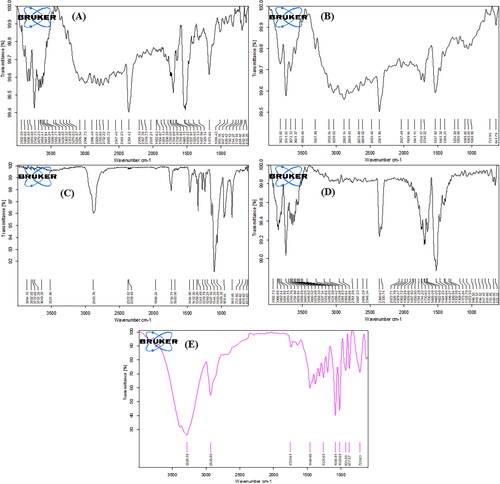
Figure 2. DSC thermogram of pure sorafenib tosylate (a), soyalecithin (B), TPGS (C), physical mixture (D), and optimized nanosuspension (formulation NSS₆) (E).

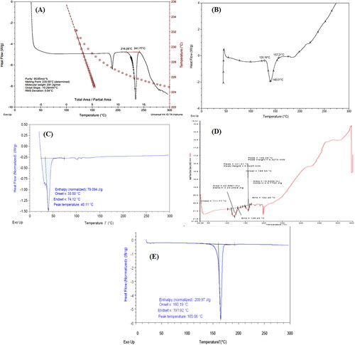
Figure 3. X-ray diffractogram of pure sorafenib tosylate (A) and optimized nanosuspension (formulation NSS₆) (B).

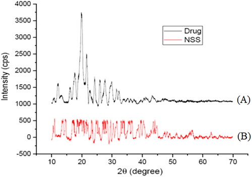
Figure 4. Scanning electron microscopic image of optimized lyophilized nanosuspension (formulation NSS₆).

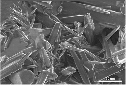
Figure 5. Particle size of formulation NSS₆ (a), pareto chart represents particle size coefficients (b1, b2, b3 are main terms; b4, b5, b6 are interaction terms and b7, b8, b9 are square terms) (B), 3D response surface (C) and contour plot (D) showing impact of various process variables on particle size.

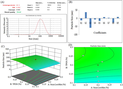
Figure 6. Zeta potential of formulation NSS₆ (a), pareto chart represent coefficients of zeta potential (b1, b2, b3 are main terms; b4, b5, b6 are interaction terms and b7, b8, b9 are square terms) (B), 3D response surface plot (C) and contour plot (D) and showing impact of various process variables on zeta potential.

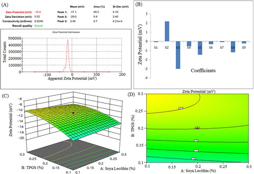
Figure 7. Pareto chart represent coefficients of drug content (b1, b2, b3 are main terms; b4, b5, b6 are interaction terms and b7, b8, b9 are square terms) (a), 3D response surface plot (B) and contour plot (C) showing impact of various process variables on drug content.

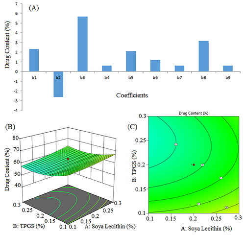
Figure 8. Pareto chart for coefficients of entrapment efficiency (b1, b2, b3 are main terms; b4, b5, b6 are interaction terms and b7, b8, b9 are square terms) (a), 3D response surface plot (B) and contour plot (C) illustrating the impact of various process variables on entrapment efficiency.

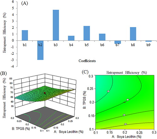
Figure 9. Pareto chart represents coefficients showing coefficients of percent cumulative drug release in 0.1 N HCl (pH 1.2) (b1, b2, b3 are main terms; b4, b5, b6 are interaction terms and b7, b8, b9 are square terms) (a), 3D response surface (B) and contour plot (C) and showing impact of various process variables on percent cumulative drug release.

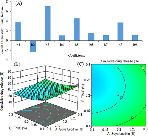
Figure 10. Pareto chart showing coefficients of percent cumulative drug release in phosphate buffer (pH 6.8) (b1, b2, b3 are main terms; b4, b5, b6 are interaction terms and b7, b8, b9 are square terms) (a), 3D response surface plot (C) and contour plot (C) illustrating the impact of various process variables on percent cumulative drug release.

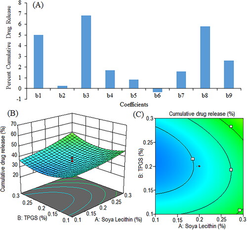
Table 3. Results Of two-way ANOVA of regression on the particle size, zeta potential, drug content, entrapment efficiency, and percent cumulative drug release in pH 1.2 and pH 6.8 dissolution media.

Response	Source of variation	Degree of freedom	Sum of squares	Mean square	F-value	P-value
Particle size	Model	9	81970.15	9107.79	4.98	0.0169*	Significant
	Residual	8	14633.81	1829.23	–
	Total	17	96603.96	–	–
Zeta potential	Model	9	226.77	25.20	15.18	0.0004*	Significant
	Residual	8	13.28	1.66	–
	Total	17	240.05	–	–
Drug content	Model	9	783.27	87.03	3.96	0.0329*	Significant
	Residual	8	175.98	22.00	–
	Total	17	959.24	–	–
Entrapment efficiency	Model	9	587.09	65.23	5.77	0.0108*	Significant
	Residual	8	90.47	11.31	–
	Total	17	677.56	–	–
Percent cumulative drug release in pH 1.2	Model	9	1322.04	146.89	4.28	0.0263*	Significant
	Residual	8	274.64	34.33	–
	Total	17	1596.68	–	–
Percent cumulative drug release in pH 6.8	Model	9	1458.82	162.09	6.49	0.0074*	Significant
	Residual	8	199.69	24.96	–
	Total	17	1658.51	–	–

Figure 11. Cumulative percentage release of sorafenib tosylate in 0.1 N HCl (pH 1.2) from the nanosuspension prepared using nanoprecipitation-sonication technique.

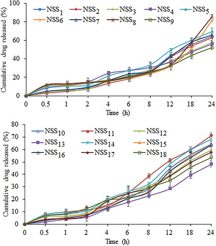
Figure 12. Cumulative percentage release of sorafenib tosylate in phosphate buffer (pH 6.8) from the nanosuspension prepared using nanoprecipitation-sonication technique.

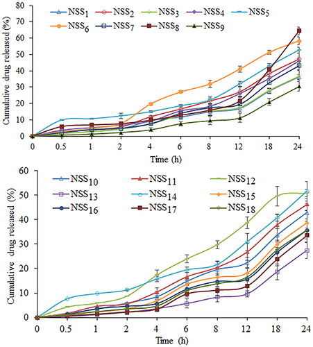
Table 4. Correlation coefficient value from different drug release kinetics.

Kinetics Model for drug release	Correlation coefficient
	0.1 N HCl (pH 1.2)	Phosphate buffer (pH 6.8)
Zero order	0.7814	0.9698
First order	0.5995	0.9338
Higuchi’s model	0.7545	0.9820
Korsemeyer-Peppas’ model	0.9470	0.8862
Korsemeyer-Peppas’ slope value (n)	0.1246	0.1295

Figure 13. Comparison of in vitro release of optimized batch and marketed formulation (Soranib, Cipla Ltd., Mumbai, India) in 0.1 N HCl and phosphate buffer.

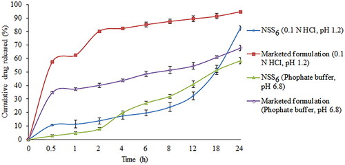
Table 5. Results of stability study of nanosuspension.

Formulation/ Parameter	Storage condition	Time period (months)
		1	2	3
Colloidal nanosuspension/ Particle size (nm)	4 ± 1 °C	100.9	109.5	116.3
	25 ± 2 °C/ 60 ± 5% RH	126.4	153.1	162.7
	45 ± 2 °C/ 75 ± 5% RH	137.6	164.9	187.4
Lyophilized nanosuspension/ Particle size (nm)	4 ± 1 °C	121.8	133.6	142.9
	25 ± 2 °C/ 60 ± 5% RH	136.5	147.2	159.6
	45 ± 2 °C/ 75 ± 5% RH	145.2	156.8	167.5
Colloidal nanosuspension/ Zeta potential (mV)	4 ± 1 °C	−18.2	−17.5	−17.9
	25 ± 2 °C/ 60 ± 5% RH	−15.7	−14.7	−13.9
	45 ± 2 °C/ 75 ± 5% RH	−12.8	−11.6	−10.3
Lyophilized nanosuspension/ Zeta potential (mV)	4 ± 1 °C	−18.7	−18.3	−17.2
	Room Temperature	−17.6	−16.6	−15.8
	45 ± 2 °C/ 75 ± 5% RH	−14.9	−13.5	−12.4

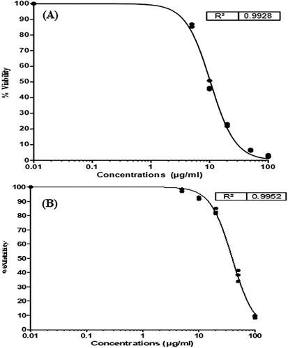
Figure 14. Results of cytotoxicity of pure sorafenib tosylate (a), and sorafenib tosylate-loaded nanosuspension (lyophilized formulation NSS6) on HepG2 cell line (B).