Behavioural processes, ephemeral resources and spring population dynamics of an insular lizard, Podarcis lilfordi (Squamata: Lacertidae)

Figures & data

Table I. Intervals between the capture–recapture occasions retained for the two analyses. The number refers to the interval in days between the current and the previous occasion. K = number of occasions retained; – = first occasion considered.

Capture–recapture occasion and date		First analysis (k = 28)	Second analysis (k = 12)
1	13 April 2004	-	-
2	14 April 2004	1	1
3	15 April 2004	1	1
4	16 April 2004	1	1
5	17 April 2004	1	1
6	18 April 2004	1	1
7	19 April 2004	1	1
8	21 April 2004	2	2
9	22 April 2004	1	1
10	25 April 2004	3	3
11	26 April 2004	1	1
12	27 April 2004	1	1
13	1 June 2004	35
14	2 June 2004	1
15	3 June 2004	1
16	4 June 2004	1
17	5 June 2004	1
18	6 June 2004	1
19	7 June 2004	1
20	8 June 2004	1
21	9 June 2004	1
22	10 June 2004	1
23	11 June 2004	1
24	8 July 2004	27
25	9 July 2004	1
26	10 July 2004	1
27	11 July 2004	1
28	15 July 2004	4

Figure 1. The proportion of females (black dots) form April to July seemed to increase. The lines (right axis) showed the number of newly marked lizards (males: dashed line, females: continuous line).

Table II. Modes and their estimates of daily survival in male and female lizards, f, and recapture probability, p. Model notation: f’ = newly marked male survival; s = sex; t = time; m = trap-dependent effect; * = interactions between effects; + = additive relationship between effects; t = trend over time; np = number of parameters. In model notation, ‘s’ to distinguish it from the daily survival denoted ‘f’ in the previous analysis. QAICc: Quasi-likelihood adjusted Akaike Information Criterion; DQAICc: Delta Quasi-likelihood adjusted Akaike Information Criterion; QDeviance: Quasi-likelihood Deviance.

Model	Notation	QAICc	DQAICc	np	QDeviance
1	f’(T)f (T*s) p(t + s + m)	3582.0582	0	35	1785.9844
4	f’(T)f (T*s) p(t + s + m)	3584.9528	2.8946	33	1793.0061
4	f’(T)f (T*s) p(t + s + m)◊	3585.6025	3.5443	34	1791.5932
5	f’(T)f (T + s) p(t + s + m)	3585.8258	3.7676	34	1791.8166
6	f’(T)f (T) p(t + s + m)	3587.1244	5.0662	33	1795.1778
8	f’(T)f (.) p(t + s + m)	3587.5441	5.4859	32	1797.6581
13	f’(.)f (.) p(t + s + m)	3614.7096	32.6514	31	1826.8824
14	f’(.)f (s) p(t + s + m)	3616.2368	34.1786	32	1826.3508
15	f’(t)f (t) p(t + s + m)◊	3618.5535	36.4953	58	1774.4703
16	f’(t)f (t + s) p(t + s + m)◊	3620.5418	38.4836	59	1774.3481
17	f(.) p(t + s + m)	3621.9075	39.8493	30	1836.1373
18	f(t + s) p(t + s + m)	3624.2074	42.1492	58	1780.1242
24	f(t) p(t + s + m)	3629.4451	47.3869	57	1787.4704
29	f(t*s) p(t + s + m)	3665.9772	83.919	84	1766.3792
30	f(.) p(s + m)	3699.1749	117.1167	5	1964.2258
31	f’(t)f (t*s)p(t + s + m)	3702.6288	120.5706	110	1746.1497
34	f (t*s)p(t*s*m)	3743.9837	161.9255	160	1674.0884
35	f’(.)f (s)p(t + s)	3767.8384	185.7802	30	1982.0682
36	f’(t)f (t*s)p(t*s*m)	3786.3452	204.287	187	1652.8888
37	f (t*s)p(t*s)	3829.7714	247.7132	108	1877.7174

◊ Trend in already marked male is assumed to be parallel to the one of already marked males.

Figure 2. A, A model assuming a linear constraint on survival as in Equation1 indicates that local daily survival decreased over time (solid line). Bars are the 95% confidence interval. B, Proportion of transient males, i.e. animals seen only at marking. Solid dots are from model f’(t) f(t*s) p(t + s + m) while the solid line indicates the expected values from the model f’(T) f(T*s) p(t + s + m).

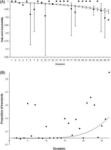
Figure 3. Frequency of gaps, i.e. number of consecutive zeros between two recapture events, in April capture–recapture data.

Table III. Models of population size and recruitment, b, during the month of April Model notation: f’ = newly marked male survival; s = sex; t = time; m = trap-dependent effect; * = interactions between effects; + = additive relationship between effects; t = trend over time; np = number of parameters. In model notation, ‘s’ to distinguish it from the daily survival denoted ‘f’ in the previous analysis (see more details in the text).

Model	AICc	DAICc	np	Model L.
f(s) p(t*s) b(t + s)	1651.238	0	36	1
f(s) p(t + s) b(t + s)	1651.303	0.06	26	0.968
f(s) p(t*s) b(t*s)	1653.748	2.51	41	0.285
f(s) p(t + s) b(t*s)	1657.462	6.22	32	0.0445
f(s) p(t*s) b(t)	1668.584	17.35	36	0.0002
f(s) p(T*s) b(t*s)	1670.543	19.31	36	0.0001
f(s) p(T*s) b(t*s)	1672.934	21.7	37	0
f(t*s) p(t*s) b(t*s)	1673.573	22.33	47	0

Figure 4. The proportion of females in the study area during the month of April, estimated by averaging the derived estimates from model f(s) p(t + s) b(t + s) and f(s) p(t*s) b(t + s). The number of individuals estimated to be present at a given time is estimated as derived parameters (see text for details).