Figures & data
Table 1. Source information and GenBank accession numbers of the studied strains.
Figure 1. Maximum likelihood phylogenetic tree inferred from combined dataset of ITS and LSU sequence data for Paracamarosporium noviaquum CNUFC MSW24-4, Pa. noviaquum CNUFC MSW24-4-1, and related species. Bootstrap support values for maximum likelihood (MLBS) higher than 70% and Bayesian posterior probabilities (BPP) greater than 0.95 are indicated above or below branches. Alloconiothyrium aptrootii CBS 980.95 was used as the outgroup. The newly generated sequences are indicated in bold blue. T = ex-type.
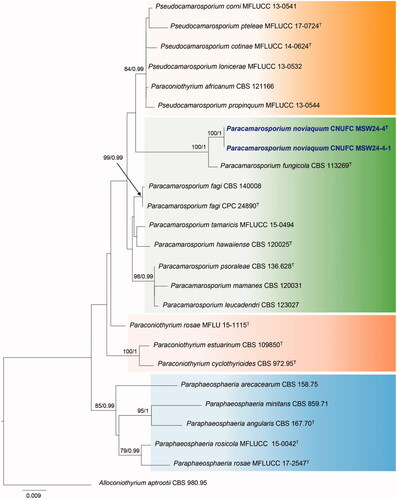
Figure 2. Maximum likelihood phylogenetic tree inferred from combined ITS, TEF1, and ACT gene sequence data for Phyllosticta gwangjuensis CNUFC NJ1-12, P. gwangjuensis CNUFC NJ1-12-1, and related species. Bootstrap support values for maximum likelihood (MLBS) higher than 70% and Bayesian posterior probabilities (BPP) greater than 0.95 are indicated above or below branches. Phyllosticta vaccinia ATCC 46255 was used as the outgroup. The newly generated sequences are indicated in bold blue. T = ex-type.
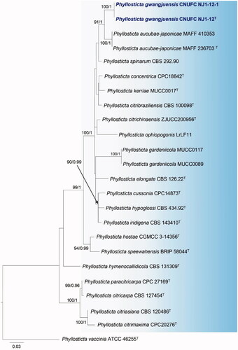
Figure 3. Maximum likelihood phylogenetic tree inferred from combined ITS and RPB2 gene sequence data for Cosmospora lavitskiae CNUFC TKB240, and related species. Bootstrap support values for maximum likelihood (MLBS) higher than 70% and Bayesian posterior probabilities (BPP) greater than 0.95 are indicated above or below branches. Nectria cinnabarina CBS 125165 was used as the outgroup. The newly generated sequences are indicated in bold blue. T = ex-type.
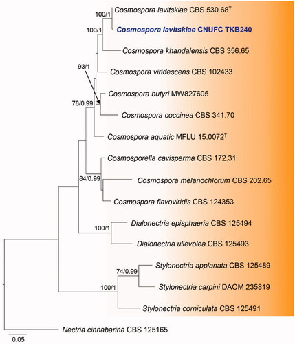
Figure 4. Maximum likelihood phylogenetic tree inferred from ITS sequence data for Monochaetia camelliae CNUFC KOW41, and related species. Bootstrap support values for maximum likelihood (MLBS) higher than 70% and Bayesian posterior probabilities (BPP) greater than 0.95 are indicated above or below branches. Distononappendiculata banksiae CBS 131308 was used as the outgroup. The newly generated sequences are indicated in bold blue. T = ex-type.
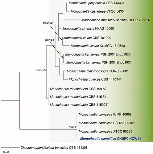
Figure 5. Maximum likelihood phylogenetic tree inferred from combined ITS and LSU sequence data for Roussoella doimaesalongensis CNUFC WT16, and related species. Bootstrap support values for maximum likelihood (MLBS) higher than 70% and Bayesian posterior probabilities (BPP) greater than 0.95 are indicated above or below branches. Setoarthopyrenia chromolaenae MFLUCC 17-1444 was used as the outgroup. The newly generated sequences are indicated in bold blue. T = ex-type.
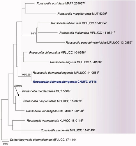
Figure 6. Morphology of Paracamarosporium noviaquum. (A) Colonies on PDA; (B) Colonies on MEA; (C) Colonies on OA; (D, E) Conidiomata on PDA; (F) Pycnidium; (G, H) Conidiogenous cells on pycnidial wall; (I) Ostiole of pycnidium; (J) 1-celled conidia; (K) 2-celled conidia; (D, E) Observed using stereo-microscope; (F–H, J, K) LM; (I) SEM) (scale bars: F = 100 μm; G, H = 20 μm, I = 40 μm; J, K = 10 μm).
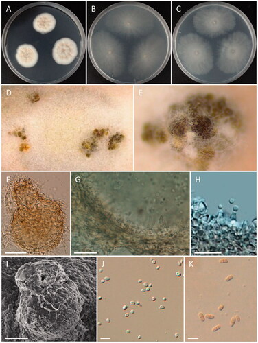
Figure 7. Morphology of Phyllosticta gwangjuensis. (A) Colonies on PDA; (B) Colonies on MEA; (C) Colonies on OA; (D) Torreya nucifera as host plant; (E, F) Conidiomata; (G–I) Conidiogenous cells and conidia; (J–M) Conidia; (L, M) SEM (scale bars: E = 2 mm; F = 1 mm; G, H = 20 μm; I–L = 10 μm; M = 5 μm).
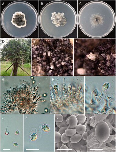
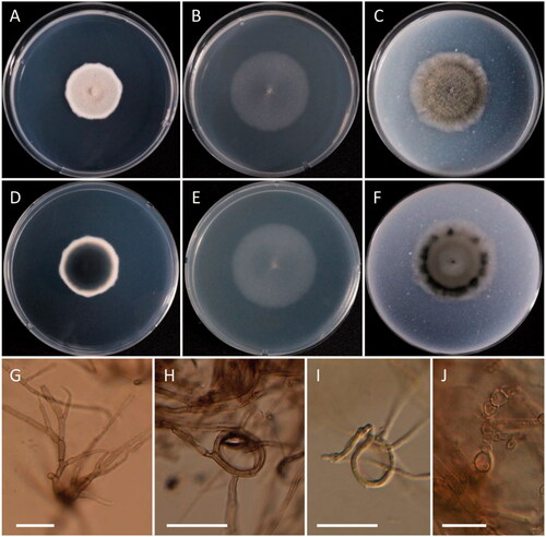
Figure 8. Morphology of Cosmospora lavitskiae. (A, D) Colonies on PDA; (B, E) Colonies on MEA; (C, F) Colonies on OA ((A–C) obverse view; (D–F) reverse view); (G–I) Phialides on conidiophores; (J) Coiled hyphae; (K) Conidia (scale bars: G–I = 20 μm; J, K = 10 μm).

Figure 9. Morphology of Monochaetia camelliae. (A, D) Colonies on PDA; (B, E) Colonies on MEA; (C, F) Colonies on OA ((A–C) obverse view; (D–F) reverse view); (G) Conidiomata; (H–K, M) Conidiogenous cells and conidia; (L) Exudate on OA; (N) Conidiomatal wall; (O) Conidia (scale bars: H–K, M–O = 10 μm).
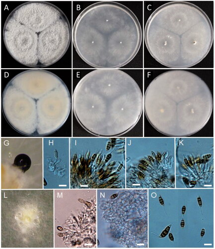
Figure 10. Morphology of Roussoella doimaesalongensis. (A, D) Colonies on PDA; (B, E) Colonies on MEA; (C, F) Colonies on OA ((A–C) obverse view; (D–F) reverse view). (G–I) Hyphae and coiled hyphae; (J) Chlamydospores (scale bars: G–I = 20 μm; J = 10 μm).