Comparison of the stabilising effects of government spending shocks in the Czech Republic, Hungary and Poland

Figures & data

Table 1. Spending multipliers: baseline model with k = 1 lag.

	Cumulative multiplier after quarter			Peak multiplier
	4th	8th	16th
Czech Republic	0.3690	0.7379	1.2089	0.1550 (4)
Hungary	0.5415	0.8167	1.0200	0.3041 (2)*
Poland	1.4638	1.6931	1.8299	1.7610 (7)*

Notes: In the case of the peak multiplier, the sign * denotes the significance of the calculation based on the error bands. The number in brackets denotes the quarter with the maximum response. The calculation of the cumulative multiplier is based on the accumulated responses, whereas the calculation of the peak multiplier is based on the responses of Y to the initial one standard deviation shock in G.

Source: Author’s own calculations.

Table 2. Spending multipliers: baseline model with k = 4 lags.

	Cumulative multiplier after quarter			Peak multiplier
	4th	8th	16th
Czech Republic	0.3409	0.8582	1.4356	0.2430 (6)
Hungary	0.6462	1.0319	1.5827	0.6725 (3)*
Poland	1.2456	1.5969	1.8798	2.2880 (7)*

Notes: In the case of the peak multiplier, the sign * denotes the significance of the calculation based on the error bands. The number in brackets denotes the quarter with the maximum response. The calculation of the cumulative multiplier is based on the accumulated responses, whereas the calculation of the peak multiplier is based on the responses of Y to the initial one standard deviation shock in G.

Source: Author’s own calculations.

Table 3. Peak spending multipliers for Poland; specifications without the ‘crisis’ dummy variable.

Baseline model, k = 1 lag	Baseline model, k = 4 lags	Model with direct taxes, k = 1 lag	Model with direct taxes, k = 4 lags	Model with indirect taxes, k = 1 lag	Model with indirect taxes, k = 4 lags
1.21 (3)*	1.80 (7)*	1.08 (3)*	2.00 (7)*	1.29 (2)*	2.06 (6)*

Notes: * denotes the significance of the calculation based on the error bands. The number in brackets denotes the quarter with the maximum response.

Source: Author’s own calculations.

Table A1. Unit root test for variables (data in log).

		Regression with trend and constant			Regression with constant, without trend
		Czech Republic	Hungary	Poland	Czech Republic	Hungary	Poland
ADF	$G_t$	–2.7206 (0.2316)	–2.8602 (0.1814)	–1.1631 (0.9088)	–2.2371 (0.1952)	–2.8059 (0.0626)	–1.7197 (0.4163)
	$R_t$	–4.7563 (0.0013)	–2.3328 (0.4112)	–2.2715 (0.4429)	–1.5394 (0.5084)	–0.8543 (0.7972)	–1.2623 (0.6420)
	$Y_t$	–1.5684 (0.7962)	–1.8707 (0.6597)	–1.6074 (0.7792)	–1.1731 (0.6821)	–1.3303 (0.6115)	–0.9159 (0.7771)
	${\Delta G}_t$	–13.8233 (0.0001)	–2.2971 (0.4297)	–3.8366 (0.0212)	–13.8347 (0.0001)	–2.2201 (0.2012)	–3.5577 (0.0096)
	${\Delta R}_t$	–14.2564 (0.0001)	–8.5978 (0.0000)	–5.4798 (0.0001)	–14.3539 (0.0001)	–8.6792 (0.0000)	–5.5089 (0.0000)
	${\Delta Y}_t$	–5.6657 (0.0001)	–4.8414 (0.0010)	–9.2605 (0.0000)	–5.6420 (0.0000)	–4.8595 (0.0001)	–9.2144 (0.0000)
PP	$G_t$	–3.6673 (0.0308)	–2.0428 (0.5686)	–1.1479 (0.9122)	–1.3144 (0.6191)	–1.9448 (0.3105)	–1.6419 (0.4556)
	$R_t$	–4.9045 (0.0008)	–6.7690 (0.0000)	–2.1944 (0.4843)	–2.0489 (0.2658)	–2.7898 (0.0645)	–1.2238 (0.6592)
	$Y_t$	–1.6519 (0.7627)	–1.9805 (0.6023)	–1.6015 (0.7816)	–1.3144 (0.6191)	–1.7172 (0.4186)	–0.9455 (0.7673)
	${\Delta G}_t$	–19.9127 (0.0001)	–9.5100 (0.0000)	–8.6616 (0.0000)	–17.0958 (0.0001)	–9.5094 (0.0000)	–8.5109 (0.0000)
	${\Delta R}_t$	–20.1116 (0.0001)	–21.7084 (0.0001)	–9.1319 (0.0000)	–20.4093 (0.0001)	–23.3750 (0.0001)	–9.2023 (0.0000)
	${\Delta Y}_t$	–5.8311 (0.0000)	–4.7965 (0.0011)	–9.1746 (0.0000)	–5.8008 (0.0000)	–4.8052 (0.0002)	–9.1204 (0.0000)

Notes: p-values in brackets, ADF – Augmented Dickey-Fuller test, PP – Phillips–Perron test, $\Delta$ refers to the first differences.

Table A2. Lag length criteria for the baseline model.

		0	1	2	3	4
AIC	Czech Republic	–8.696246	–12.01446*	–11.97899	–11.89634	–11.85934
	Hungary	–9.128542	–12.03836*	–11.94079	–11.73642	–11.82031
	Poland	–12.05529	–15.09811*	–14.99771	–14.90429	–14.83318
SIC	Czech Republic	–8.395177	–11.41232*	–11.07579	–10.69206	–10.35400
	Hungary	–8.827473	–11.43623*	–11.03758	–10.53215	–10.31497
	Poland	–11.74385	–14.47523*	–14.06339	–13.65853	–13.27598
HQC	Czech Republic	–8.577455	–11.77687*	–11.62262	–11.42117	–11.26539
	Hungary	–9.009751	–11.80078*	–11.58442	–11.26126	–11.22636
	Poland	–11.93324	–14.85400*	–14.63154	–14.41606	–14.22290

Notes: * Denotes the lag order selected by the criterion, AIC – Akaike information criterion, SIC – Schwarz information criterion, HQC – Hannan–Quinn information criterion.

Table A3. Elements of A and B matrices for the baseline model.

	$a_4$	$a_5$	$b_1$	$b_2$	$b_4$	$b_3$	$a_6$
Czech Republic	0.018 (0.529)	–0.002 (0.894)	0.058 (0.000)	0.009 (0.000)	0.070 (0.000)	0.061 (0.000)	0.96
Hungary	0.044 (0.040)	0.002 (0.855)	0.042 (0.000)	0.007 (0.000)	–0.016 (0.202)	0.099 (0.000)	0.98
Poland	0.230 (0.000)	–0.012 (0.479)	0.016 (0.000)	0.007 (0.000)	0.013 (0.054)	0.054 (0.000)	1.15

Notes: p-values in brackets; ${\mathrm{a}}_6$ is exogenously-calculated average elasticity.

Table A4. Elements of A and B matrices – model with direct taxes, k = 1 lag.

	$a_4$	$a_5$	$b_1$	$b_2$	$b_4$	$b_3$	$a_6$
Czech Republic	0.021 (0.257)	–0.004 (0.950)	0.059 (0.000)	0.009 (0.000)	0.001 (0.999)	0.019 (0.000)	0.27
Hungary	0.091 (0.009)	–0.031 (0.127)	0.029 (0.000)	0.007 (0.000)	0.019 (0.001)	0.045 (0.000)	0.29
Poland*	×	×	×	×	×	×	0.05

Notes: p-values in brackets; ${\mathrm{a}}_6$ is exogenously-calculated average elasticity.

* In the case of Poland, x denotes a lack of satisfactory models.

Table A5. Elements of A and B matrices – model with direct taxes, k = 4 lags.

	$a_4$	$a_5$	$b_1$	$b_2$	$b_4$	$b_3$	$a_6$
Czech Republic	0.015 (0.359)	–0.007 (0.891)	0.062 (0.000)	0.008 (0.000)	0.001 (0.796)	0.019 (0.000)	0.27
Hungary	0.073 (0.066)	–0.021 (0.298)	0.024 (0.000)	0.007 (0.000)	0.014 (0.018)	0.045 (0.000)	0.29
Poland	0.224 (0.000)	0.072 (0.035)	0.015 (0.000)	0.007 (0.000)	0.003 (0.350)	0.025 (0.000)	0.05

Notes: p-values in brackets; ${\mathrm{a}}_6$ is exogenously-calculated average elasticity.

Table A6. Elements of A and B matrices – model with indirect taxes, k = 1 lag.

	$a_4$	$a_5$	$b_1$	$b_2$	$b_4$	$b_3$	$a_6$
Czech Republic	0.026 (0.125)	0.101 (0.003)	0.059 (0.000)	0.009 (0.000)	–0.003 (0.341)	0.029 (0.000)	0.34
Hungary	0.116 (0.001)	0.044 (0.050)	0.029 (0.000)	0.007 (0.000)	–0.011 (0.037)	0.040 (0.000)	0.45
Poland	0.179 (0.001)	0.025 (0.124)	0.016 (0.000)	0.007 (0.000)	0.013 (0.036)	0.048 (0.000)	0.87

Notes: p-values in brackets; ${\mathrm{a}}_6$ is exogenously-calculated average elasticity.

Table A7. Elements of A and B matrices – model with indirect taxes, k = 4 lags.

	$a_4$	$a_5$	$b_1$	$b_2$	$b_4$	$b_3$	$a_6$
Czech Republic	0.024 (0.130)	0.098 (0.003)	0.062 (0.000)	0.008 (0.000)	–0.004 (0.284)	0.029 (0.000)	0.34
Hungary*	×	×	×	×	×	×	0.45
Poland	0.213 (0.001)	0.016 (0.369)	0.015 (0.000)	0.007 (0.000)	0.016 (0.007)	0.046 (0.000)	0.87

Notes: p-values in brackets; ${\mathrm{a}}_6$ is exogenously-calculated average elasticity.

* In the case of Hungary, × denotes a lack of satisfactory models.

Table A8. Elements of A and B matrices – the baseline model with 4 lags.

	$a_4$	$a_5$	$b_1$	$b_2$	$b_4$	$b_3$	$a_6$
Czech Republic	0.012 (0.664)	0.001 (0.966)	0.063 (0.000)	0.008 (0.000)	0.076 (0.000)	0.055 (0.000)	0.96
Hungary	0.077 (0.025)	–0.005 (0.583)	0.025 (0.000)	0.007 (0.000)	–0.012 (0.316)	0.098 (0.000)	0.98
Poland	0.249 (0.001)	–0.020 (0.249)	0.016 (0.000)	0.007 (0.000)	0.010 (0.159)	0.056 (0.000)	1.15

Notes: p-values in brackets; ${\mathrm{a}}_6$ is exogenously-calculated average elasticity.

Table A9. Elements of A and B matrices – subsample since 2007.

	$a_4$	$a_5$	$b_1$	$b_2$	$b_4$	$b_3$	$a_6$
Czech Republic*	×	×	×	×	×	×	0.96
Hungary	0.166 (0.072)	0.006 (0.802)	0.027 (0.000)	0.009 (0.000)	0.037 (0.000)	0.061 (0.000)	0.98
Poland	0.235 (0.001)	0.016 (0.519)	0.017 (0.000)	0.007 (0.000)	0.005 (0.448)	0.043 (0.000)	1.15

Notes: p-values in brackets; ${\mathrm{a}}_6$ is exogenously-calculated average elasticity.

* In the case of the Czech Republic, × denotes a lack of satisfactory models.

Table A10. Peak multipliers (adjusted to be interpreted in the national currency) in robust system specifications.

	Direct taxes	Indirect taxes	Direct taxes, k = 4 lags	Indirect taxes, k = 4 lags	Baseline model, k = 4 lags	Baseline model, sample since 2007
Czech Republic	0.1753 (3)	0.1719 (3)	0.2453 (6)	0.3429 (6)*	0.2430 (6)	×
Hungary	0.4529 (4)*	0.8514 (7)*	0.4602 (5)	×	0.6725 (3)*	0.6774 (7)
Poland	×	1.8335 (7)*	2.1727 (7)*	2.2655 (7)*	2.2880 (7)*	1.0744 (1)*

Notes: * Denotes significance based on the error bands; the quarter with the peak value is in brackets; × indicates a lack of satisfactory models.

Table A11. Elements of A and B matrices, the additional SVAR specification for Poland.

	$a_4$	$a_5$	$b_1$	$b_2$	$b_4$	$b_3$	$a_6$
baseline model, k = 1 lag	0.206 (0.000)	0.009 (0.555)	0.016 (0.000)	0.007 (0.000)	0.013 (0.088)	0.059 (0.000)	1.15
baseline model, k = 4 lags	0.219 (0.001)	0.001 (0.988)	0.016 (0.000)	0.001 (0.000)	0.011 (0.166)	0.061 (0.000)	1.15
model with direct taxes, k = 1 lag	0.184 (0.001)	0.091 (0.001)	0.016 (0.000)	0.007 (0.000)	0.003 (0.412)	0.034 (0.000)	0.05
model with direct taxes, k = 4 lags	0.221 (0.000)	0.099 (0.001)	0.015 (0.000)	0.006 (0.000)	0.003 (0.337)	0.029 (0.000)	0.05
model with indirect taxes, k = 1 lag	0.166 (0.002)	0.042 (0.008)	0.016 (0.000)	0.007 (0.000)	0.013 (0.045)	0.051 (0.000)	0.87
model with indirect taxes, k = 4 lags	0.194 (0.002)	0.029 (0.096)	0.015 (0.000)	0.007 (0.000)	0.015 (0.010)	0.047 (0.000)	0.87

Notes: p-values in brackets; ${\mathrm{a}}_6$ is exogenously-calculated average elasticity.

Figure A1. Inverse roots of AR Characteristic Polynomial for baseline model.

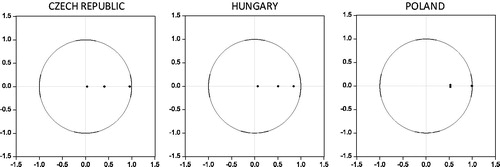
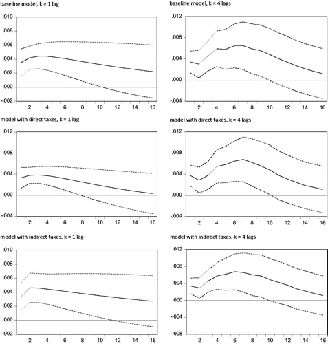
Figure A2. Impulse responses of Y to structural one s.d. shock in G ± 2 s.e., baseline model.

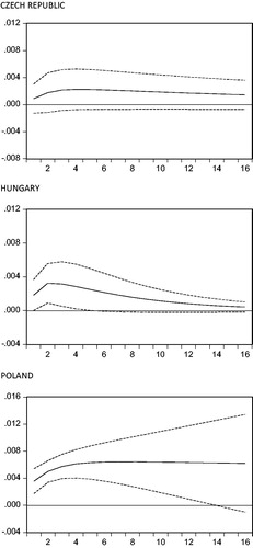
Figure A3. Impulse responses of Y to structural one s.d. shock in G ± 2 s.e., model with direct taxes, k = 1 lag.

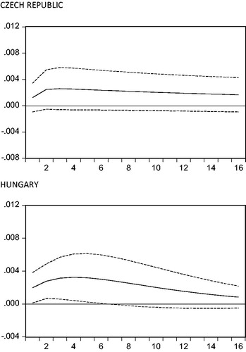
Figure A4. Impulse responses of Y to structural one s.d. shock in G ± 2 s.e., model with direct taxes, k = 4 lags.

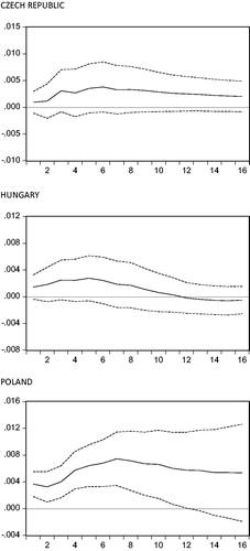
Figure A5. Impulse responses of Y to structural one s.d. shock in G ± 2 s.e., model with indirect taxes, k = 1 lag.

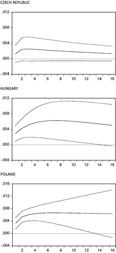
Figure A6. Impulse responses of Y to structural one s.d. shock in G ± 2 s.e., model with indirect taxes, k = 4 lags.

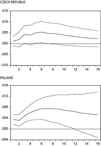
Figure A7. Impulse responses of Y to structural one s.d. shock in G ± 2 s.e., baseline SVAR with k = 4 lags.

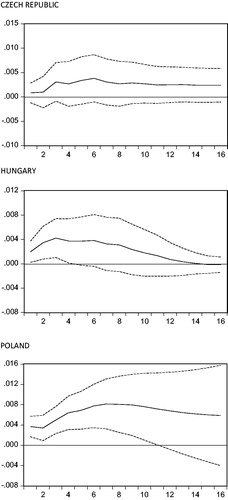
Figure A8. Impulse responses of Y to structural one s.d. shock in G ± 2 s.e., subsample since 2007.

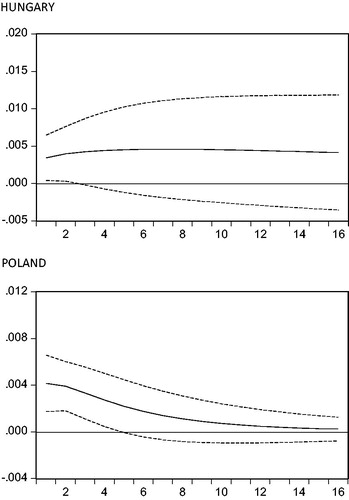
Figure A9. Impulse responses of Y to structural one s.d. shock in G ± 2 s.e. for Poland, SVAR specifications without the dummy variable for the crisis and post-crisis period.