Dynamic behaviour of optimal portfolio with stochastic volatility

Figures & data

Figure 1. Time-dependent paths of (a) mean, and (b) variance of the optimal weight ${\pi }^{*}(t)$ for the risky asset under three different mean reversion speed κ, with model parameters: ${\pi }^{*}(0)=0.6,v(0)=0.02<\theta =0.04,\sigma =0.02.$ Source: The authors.

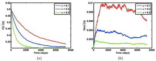
Figure 2. Time-dependent paths of (a) mean, and (b) variance of the optimal weight ${\pi }^{*}(t)$ for the risky asset under three different mean reversion speed κ, with model parameters: ${\pi }^{*}(0)=0.6,v(0)=0.06>\theta =0.04,\sigma =0.02.$ Source: The authors.

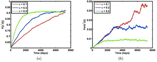
Figure 3. Time-dependent paths of (a) mean, and (b) variance of the optimal weight ${\pi }^{*}(t)$ for the risky asset under three different long-run variance θ, with model parameters: ${\pi }^{*}(0)=0.6,v(0)=0.02,\kappa =0.2,\sigma =0.02.$ Source: The authors.

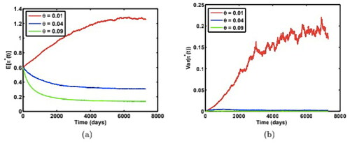
Figure 4. Time-dependent paths of (a) mean, and (b) variance of the optimal weight ${\pi }^{*}(t)$ for the risky asset under three different long-run variance θ, with model parameters: ${\pi }^{*}(0)=0.6,v(0)=0.06,\kappa =0.2,\sigma =0.02.$ Source: The authors.

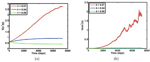
Figure 5. Time-dependent paths of (a) mean, and (b) variance of the optimal weight ${\pi }^{*}(t)$ for the risky asset under three different volatility of volatility σ, with model parameters: ${\pi }^{*}(0)=0.6,v(0)=0.02<\theta =0.04,\kappa =0.2.$ Source: The authors.

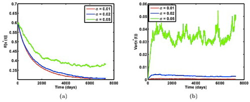
Figure 6. Time-dependent paths of (a) mean, and (b) variance of the optimal weight ${\pi }^{*}(t)$ for the risky asset under three different volatility of volatility σ, with model parameters: ${\pi }^{*}(0)=0.6,v(0)=0.06>\theta =0.04,\kappa =0.2.$ Source: The authors.

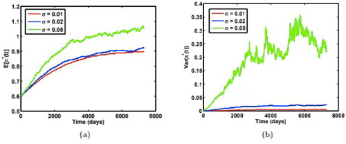
Figure 7. Comparison of (a) mean weight paths, and (b) variance of weight paths from two numerical simulation methods to test for robustness, with model parameters: ${\pi }^{*}(0)=0.6,v(0)=0.02<\theta =0.04,\kappa =0.1,\sigma =0.02.$ Source: The authors.

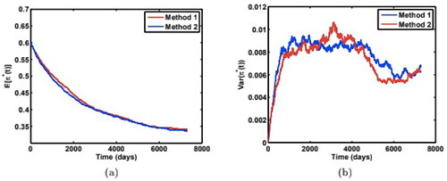
Figure 8. Comparison of (a) mean weight paths, and (b) variance of weight paths from two numerical simulation methods to test for robustness, with model parameters: ${\pi }^{*}(0)=0.6,v(0)=0.02<\theta =0.04,\kappa =0.2,\sigma =0.02.$ Source: The authors.

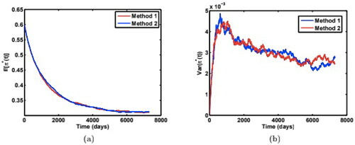
Figure 9. Comparison of (a) mean weight paths, and (b) variance of weight paths from two numerical simulation methods to test for robustness, with model parameters: ${\pi }^{*}(0)=0.6,v(0)=0.02<\theta =0.04,\kappa =0.5,\sigma =0.02.$ Source: The authors.

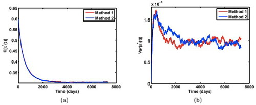
Figure 10. Comparison of (a) mean paths of weights, and (b) variance of weight paths from simulations using two different time steps (daily v.s. monthly) with model parameters: ${\pi }^{*}(0)=0.6,v(0)=0.02<\theta =0.04,\kappa =0.2,\sigma =0.02.$ Source: The authors.

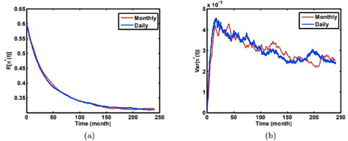
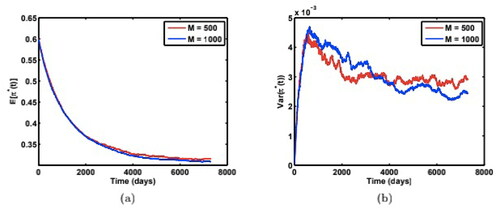
Figure 11. Comparison of (a) mean paths of weights, and (b) variance of weight paths from numerical simulations (method 1) for two different numbers of Monte Carlo simulation paths (M = 500 v.s. 1000) with model parameters: ${\pi }^{*}(0)=0.6,v(0)=0.02<\theta =0.04,\kappa =0.2,\sigma =0.02.$ Source: The authors.

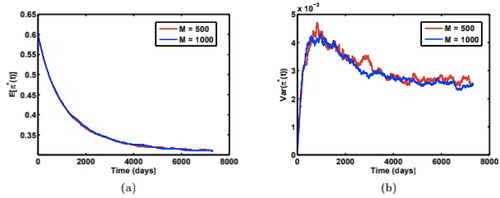
Figure 12. Comparison of (a) mean paths of weights, and (b) variance of weight paths from numerical simulations (method 2) for two different numbers of Monte Carlo simulation paths (M = 500 v.s. 1000) with model parameters: ${\pi }^{*}(0)=0.6,v(0)=0.02<\theta =0.04,\kappa =0.2,\sigma =0.02.$ Source: The authors.