Environmental regulation and sectoral disparity in labor demand: evidence from a quasi-natural experiment in China

Figures & data

Figure 1. Geographical distribution of TCZ and non-TCZ cities.

Notes: This figure shows the geographical distribution of TCZ and non-TCZ cities in China. The dark red, light red, and white regions are ARCZ, SPCZ, and non-TCZ cities, respectively.

Source: “The Official Reply of the State Council Concerning Acid Rain Control Zones and Sulfur Dioxide Pollution Control Zones”.

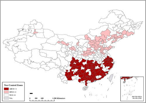
Figure 2. The difference in $S{O}_2$ emission reduction between TCZ and non-TCZ cities.

Notes: This figure plots the distribution of $S{O}_2$ emission reduction (log) of industrial enterprises in TCZ and non-TCZ cities in the year when the TCZ policy was issued and ended.

Source: China Environmental Statistics Database in 1998 and 2010.

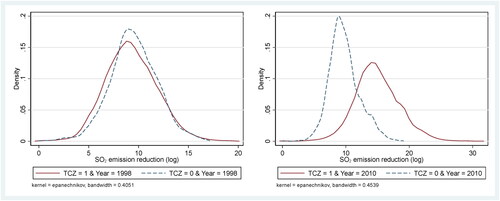
Table 1. Summary statistics.

Variables	Description	Treatment group			Control group
		Obs.	Mean	SD	Obs.	Mean	SD
Panel A. Enterprise-level variables
Output	Log of industrial value added	243,547	8.910	1.574	77,847	8.644	1.671
Labor	Log of no. of employees	243,547	5.501	1.232	77,847	5.515	1.258
Size	Log of total assets	243,547	10.390	1.361	77,847	10.219	1.372
Wage	Log of per-capita wages	243,547	2.018	0.922	77,847	1.664	0.918
Age	Log of firm age	243,547	2.732	0.844	77,847	2.874	0.862
Tax	Ratio of tax payment to revenue	243,547	0.082	2.037	77,847	0.087	1.489
Export	Ratio of export to revenue	243,547	0.202	6.200	77,847	0.089	1.208
Leverage	Ratio of liability to asset	243,547	0.675	0.360	77,847	0.753	0.391
Turnover	Ratio of revenue to asset	243,547	0.901	1.335	77,847	0.788	1.337
ROA	Return on assets	243,547	0.014	0.127	77,847	0.008	0.105
Multi	= 1(Business unit > 1)	243,547	0.036	0.187	77,847	0.062	0.241
SOEs	= 1(State-owned enterprise)	243,547	0.309	0.462	77,847	0.501	0.500
Private	= 1(Private enterprise)	243,547	0.483	0.500	77,847	0.446	0.497
FIEs	= 1(Foreign-invested enterprise)	243,547	0.208	0.406	77,847	0.053	0.224
Panel B. Industry-level variables
$S{O}_{2,03-06}$	$S{O}_2$ emission intensity (2003–2006, average)	243,547	0.052	0.106	77,847	0.075	0.146
$S{O}_{2,1995}$	$S{O}_2$ emission intensity in 1995	117,570	0.674	1.466	37,725	1.067	2.176
$S{O}_{2,\mathit{high}}$	= 1(Emission-intensive industry)	243,547	0.405	0.491	77,847	0.525	0.499
$N{H}_{3,03-06}$	$N{H}_3$ emission intensity (2003–2006, average)	243,547	0.015	0.063	77,847	0.024	0.093
Panel C. City-level variables
${\mathit{FDI}}_{90-95}$	Log of the FDI inflows (1990–1995, average)	234,174	9.365	1.828	63,564	7.028	1.453

Notes: All nominal variables are deflated at the province level (year 1995 = 100). Emission-intensive industries are defined as the ones whose $S{O}_2$ emissions accounted for more than 1% in 1998.

Source: Sample data in this paper.

Figure 3. Checks on the identification assumption with the city-level data.

Notes: This figure illustrates the time trend of the number of total and industrial employees in TCZ and non-TCZ cities during the period from 1994 to 2006.

Source: China City Statistical Yearbook, various years.

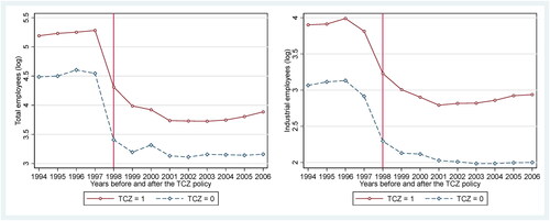
Figure 4. Checks on the identification assumption with the raw data.

Notes: This figure shows the number of averaged employees in TCZ and non-TCZ cities over time and that across industries with high/low $S{O}_2$ emission levels in the two groups of cities.

Source: Sample data in this paper.

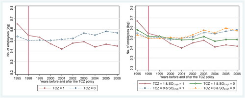
Table 2. Main results: DiD specification.

Dep. Var	Output			Labor
	(1)	(2)	(3)	(4)	(5)	(6)
$\mathit{TCZ}\times \mathit{Post}$	−0.097** (0.044)	−0.097** (0.041)	−0.134*** (0.045)	−0.275*** (0.052)	−0.259*** (0.051)	−0.231*** (0.052)
TCZ	0.314*** (0.062)			0.105 (0.138)
Post	−0.111*** (0.037)			−0.153*** (0.032)
Size			0.872*** (0.004)			0.703*** (0.005)
Wage			0.152*** (0.010)			−0.417*** (0.015)
Age			−0.024*** (0.005)			0.171*** (0.007)
Tax			2.218*** (0.088)			1.856*** (0.073)
Export			0.122*** (0.012)			0.533*** (0.026)
Leverage			−0.168*** (0.013)			−0.078*** (0.012)
Turnover			0.644*** (0.011)			0.294*** (0.012)
ROA			2.640*** (0.064)			−0.873*** (0.064)
_cons	8.765*** (0.052)	8.912*** (0.026)	−1.057*** (0.057)	5.301*** (0.027)	5.659*** (0.033)	−1.674*** (0.075)
City F.E.		Y	Y		Y	Y
Year F.E.		Y	Y		Y	Y
Observations	321,394	321,394	321,394	321,394	321,394	321,394
Adjusted R-squared	0.007	0.079	0.737	0.002	0.040	0.647

Notes: Robust standard errors are reported in parenthesis and are clustered at the city level. ^*p < 0.1, ^**p < 0.05, ^***p < 0.01.

Source: Sample data in this paper.

Table 3. Main results: DDD specification.

Dep. Var	Output			Labor
	(1)	(2)	(3)	(4)	(5)	(6)
$\mathit{TCZ}\times \mathit{Post}\times S{O}_{2,03-06}$	−0.699*** (0.221)	−1.510** (0.600)	−1.485*** (0.518)	−0.217 (0.340)	−1.108** (0.550)	−1.433*** (0.534)
TCZ × Post	−0.028 (0.031)	−0.072* (0.043)		−0.273*** (0.040)	−0.156*** (0.040)
$\mathit{TCZ}\times S{O}_{2,03-06}$	0.547** (0.239)	1.462** (0.601)		−0.106 (0.301)	0.882 (0.550)
$\mathit{Post}\times S{O}_{2,03-06}$	1.965*** (0.170)	2.342*** (0.561)		0.407 (0.274)	−0.680*** (0.023)
TCZ	0.263*** (0.033)			0.117 (0.165)
Post	−0.242*** (0.026)			−0.138*** (0.034)
$S{O}_{2,03-06}$	−1.581*** (0.179)			−0.375 (0.239)
Size		0.875*** (0.003)	0.873*** (0.003)		0.715*** (0.003)	0.709*** (0.003)
Wage		0.159*** (0.005)	0.154*** (0.005)		−0.414*** (0.006)	−0.405*** (0.006)
Age		−0.023*** (0.003)	−0.017*** (0.003)		0.159*** (0.004)	0.154*** (0.004)
Tax		2.030*** (0.060)	1.940*** (0.064)		1.515*** (0.057)	1.417*** (0.057)
Export		0.095*** (0.010)	0.098*** (0.010)		0.382*** (0.014)	0.345*** (0.014)
Leverage		−0.180*** (0.010)	−0.178*** (0.010)		−0.068*** (0.009)	−0.053*** (0.009)
Turnover		0.644*** (0.006)	0.633*** (0.006)		0.310*** (0.005)	0.299*** (0.005)
ROA		2.561*** (0.043)	2.522*** (0.043)		−1.027*** (0.042)	−0.886*** (0.041)
_cons	8.865*** (0.027)	−1.263*** (0.063)	−1.091*** (0.038)	5.330*** (0.029)	−1.888*** (0.059)	−1.794*** (0.039)
Industry F.E.		Y			Y
City F.E.		Y			Y
Year F.E.		Y			Y
Industry-city F.E.			Y			Y
Industry-year F.E.			Y			Y
City-year F.E.			Y			Y
Observations	321,394	321,394	321,394	321,394	321,394	321,394
Adjusted R-squared	0.009	0.740	0.761	0.003	0.683	0.725

Notes: Robust standard errors are reported in parenthesis and are clustered at the industry-city level. ^*p < 0.1, ^**p < 0.05, ^***p < 0.01.

Source: Sample data in this paper.

Figure 5. Event-time estimates on labor demand before and after the TCZ policy.

Notes: Plotted are event-time estimates with our preferred setting for the state- and non-state-owned enterprises. The solid line captures the time course of the difference in firms’ labor demand between treatment and control groups. The dashed lines represent the 95% confidence intervals.

Source: Sample data in this paper.

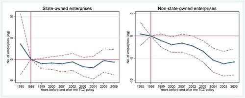
Table 4. Heterogeneity across firm ownership types.

Dep. Var: Labor	(1)	(2)	(3)
	SOEs	Private	FIEs
$\mathit{TCZ}\times \mathit{Post}\times S{O}_{2,03-06}$	0.081 (0.109)	−3.588** (1.778)	−0.322 (0.653)
Industry-city F.E.	Y	Y	Y
Industry-year F.E.	Y	Y	Y
City-year F.E.	Y	Y	Y
Observations	114,211	152,357	54,826
Adjusted R-squared	0.796	0.696	0.728

Notes: For saving space, a constant term and all controls are not reported in these regressions. Robust standard errors are reported in parenthesis and are clustered at the industry-city level. *p < 0.1, **p < 0.05, ***p < 0.01.

Source: Sample data in this paper.

Table 5. Heterogeneity across control zone types.

Dep. Var: Labor	(1)	(2)	(3)
	SPCZ	ARCZ	Pooled
$\mathit{SPCZ}\times \mathit{Post}\times S{O}_2$	0.220 (0.856)		−0.237 (0.653)
$\mathit{ARCZ}\times \mathit{Post}\times S{O}_2$		−1.618*** (0.519)	−1.601*** (0.522)
Industry-city F.E.	Y	Y	Y
Industry-year F.E.	Y	Y	Y
City-year F.E.	Y	Y	Y
Observations	153,621	245,620	321,394
Adjusted R-squared	0.739	0.723	0.725

Notes: For saving space, a constant term and all controls are not reported in these regressions. Robust standard errors are reported in parenthesis and are clustered at the industry-city level. *p < 0.1, **p < 0.05, ***p < 0.01.

Source: Sample data in this paper.

Table 6. Robustness checks.

Dep. Var: Labor	(1)	(2)	(3)	(4)	(5)	(6)
	$S{O}_{2,1995}$	$S{O}_{2,\mathit{high}}$	Falsified	Placebo	IV: 2nd	One-unit
$\mathit{TCZ}\times \mathit{Post}\times S{O}_{2,1995}$	−0.225*** (0.047)
$\mathit{TCZ}\times \mathit{Post}\times S{O}_{2,\mathit{high}}$		−0.130*** (0.048)
$\mathit{TCZ}\times \mathit{Post}\times N{H}_{3,03-06}$			−0.275 (2.035)
$\mathit{TCZ}\times \mathit{Post}\times S{O}_{2,03-06}$				0.002 (0.052)	−6.237*** (1.665)	−1.436*** (0.550)
Observations	155,295	321,394	321,394	321,394	297,738	307,725
Adjusted R-squared	0.714	0.725	0.725		0.626	0.717
Dep. Var: $\mathit{TCZ}\times \mathit{Post}\times S{O}_{2,03-06}$					IV: 1st
${\mathit{FDI}}_{90-95}\times \mathit{Post}\times S{O}_{2,03-06}$					0.107*** (0.022)
Kleibergen-Paaprk LM Statistic					15.282
Kleibergen-Paaprk Wald F Statistic					23.136
Observations					297,738
Adjusted R-squared					0.887
Industry-city F.E.	Y	Y	Y	Y	Y	Y
Industry-year F.E.	Y	Y	Y	Y	Y	Y
City-year F.E.	Y	Y	Y	Y	Y	Y

Notes: Robust standard errors are reported in parenthesis and are clustered at the industry-city level. *p < 0.1, **p < 0.05, ***p < 0.01.

Source: Sample data in this paper.

Figure 6. Distribution of estimates and t-statistics in the randomization test.

Notes: This randomization exercise is repeated 500 times and the resulting estimates and t-statistics are plotted. The red line marks the position of t-statistic for our benchmark estimate. Share is the percentage of t-statistics that is larger than the actual one.

Source: Sample data in this paper.

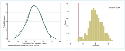
Figure 7. Temporal and spatial distribution of employees in multi- and one-unit enterprises.

Notes: Plotted is the annual average number of employees (log) in TCZ and non-TCZ cities across multi- and one-unit enterprises, respectively.

Source: Sample data in this paper.

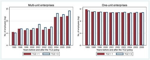
Table A1. A glossary of technical terms and abbreviations.

Category	Abbreviation	Full name
Regions	TCZ	Two Control Zones of China
	SPCZ	Sulfur Dioxide Pollution Control Zones of China
	ARCZ	Acid Rain Control Zones of China
	SCAQMD	South Coast Air Quality Management District of California, U.S.
Methods	DDD	Difference-in-Difference-in-Differences
	DiD	Difference-in-Differences
	IV	Instrumental Variable
Pollutants	SO2	Sulfur Dioxide
	NH3	Ammonia Nitrogen
Agencies	NBS	National Bureau of Statistics of China
	EPA	Environmental Protection Agency of U.S.
Standards	NAAQS	National Ambient Air Quality Standards of U.S.
	MACT	Most Achievable Control Technology Standards of U.S.
	BAT	Best Available Control Technology Standards of U.S.

Notes: This table should be put in the appendix.