Changes in radiation interception and R:FR over time and with canopy depth of two soybean cultivars with different branching characteristics

Figures & data

Figure 1. Schematic curve of a logistic function [Equation (1(1) )] fitted to the increase in FIPAR or LAI or the reduction of R:FR over time (DAS) or distance (cm) from the top of the canopy. A_upper, upper asymptote; A_low, lower asymptote; Onset and End, beginning and completion of increase (or decrease). Duration (or distance) of increase (or decrease) is DAS or distance (cm) from Onset to End (t₁ − t₀).

Figure 2. Schematic curve of an exponential function [Equation (2(2) )] fitted to the relationships between R:FR and TransPAR (– · –) and LAI ( – ).

Table 1. Monthly mean temperatures, daily total solar radiation, and precipitation during the experiments in 2014 and 2015, and the 13-year means (2001–2013) at the study site.

Month	Mean temperature (°C)			Daily total solar radiation (MJ m^−2 d^−1)			Precipitation (mm)
	2014	2015	Mean	2014	2015	Mean	2014	2015	Mean
July	26.8	25.8*	26.8	19.0	16.5^*	19.7	83*	229*	137
August	25.9*	27.1*	27.8	12.9*	17.9*	20.9	511*	154	110
September	22.8*	22.0*	24.1	16.0	13.5*	16.2	77	119	140
October	17.9	17.0*	18.2	12.1*	14.7*	12.7	244*	26*	95
E–H^a	23.4	23.2	–	1,429	1,623	–	835	463	–

* Outside of the 95% confidence interval for the 13-y mean.

^a Average of mean temperature, total daily total solar radiation, or total precipitation from emergence to the day before harvest.

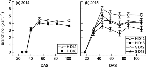
Figure 3. Changes in the number of branches per plant of Hatsusayaka (H) or Sachiyutaka (S) at normal (D12) and high (D18) densities in (a) 2014 and (b) 2015. Values are mean ± S.E. (n = 6).

Table 2. Numbers of branches and sub-branches per plant at maturity.

Year	Density	Cultivar	Branch number per plant	Sub-branch number per plant
2014	D12	Hatsusayaka	4.4 ± 0.1	4.3 ± 0.3
	D18		3.7 ± 0.1	4.0 ± 0.4
t-test			***	ns
2015	D12	Hatsusayaka	5.1 ± 0.2	5.0 ± 0.2
		Sachiyutaka	4.4 ± 0.3	4.6 ± 0.2
	D18	Hatsusayaka	4.1 ± 0.3	4.6 ± 0.3
		Sachiyutaka	3.2 ± 0.4	3.7 ± 0.2
ANOVA	Cultivar (C)		*	*
	Density (D)		**	*
	C × D		ns	ns

* p < 0.05

** p < 0.01

*** p < 0.001

Note: Mean ± S.E. (n = 6). ns, not significant.

Table 3. Onset, End, duration, and asymptote of sigmoidal curves of LAI, FIPAR, and R:FR over time at normal (D12) and high (D18) plant densities in 2014 and 2015.

	Year			2014		2015
	Treatment			D12	D18	D12		D18
	Cultivar			Hatsusayaka	Hatsusayaka	Hatsusayaka	Sachiyutaka	Hatsusayaka	Sachiyutaka
Onset		x^a	R:FR	29.9	29.9	24.1	24.4	24.8	17.7
			FIPAR	28.8	31.3	23.0	20.6	20.6	19.9
			LAI	30.7	30.1	28.0	27.4	27.8	25.5
		y	R:FR	1.045	0.923	1.04	1.032	0.995	1.096
			FIPAR	0.379	0.537	0.178	0.149	0.196	0.210
			LAI	0.89	1.19	0.94	0.82	1.16	0.93
End		x	R:FR	48.1	45.0	39.6	39.9	37.9	44.5
			FIPAR	43.6	42.1	37.2	38.8	36.0	37.0
			LAI	53.8	52.7	47.3	49.4	46.2	48.3
		y	R:FR	0.289	0.235	0.218	0.254	0.198	0.230
			FIPAR	0.903	0.926	0.898	0.89	0.905	0.901
			LAI	6.79	7.35	8.3	7.32	9.12	7.90
Duration (d)			R:FR	18.2	15.1	15.5	15.5	13.1	26.9
			FIPAR	14.8	10.8	14.2	18.2	15.4	17.2
			LAI	23.2	22.6	19.2	22.0	18.4	22.7
Asymptote		Lower	R:FR	0.194	0.149	0.115	0.157	0.099	0.122
		Upper	FIPAR	0.969	0.975	0.988	0.982	0.993	0.988
		Upper	LAI	7.53	8.12	9.22	8.14	10.12	8.77
RMSE			R:FR	0.028	0.020	0.046	0.058	0.048	0.047
			FIPAR	0.008	0.007	0.006	0.012	0.001	0.002
			LAI	0.119	0.277	0.184	0.102	0.104	0.152

^a x and y in the second culm represents the value (y) of R: FR, FIPAR, LAI and the timing (x) in DAS (d) at the Onset and End (see Figure 1).

Figure 4. Changes in (a–c) R:FR, (d–f) fraction of intercepted PAR (FIPAR), and (g–i) LAI over time in the canopy of Hatsusayaka (H) and Sachiyutaka (S) plants grown at normal (D12) and high (D18) densities in 2014 and 2015. Values are mean ± S.E. (n = 6). All variables were fitted to a logistic function [Equation (1(1) )]. The Onset and End (x and y), duration, asymptote, and root mean square error of the fitted lines are shown in Table 3.

Table 4. Pearson’s correlation coefficients (r) for the relationships between Onset, End, asymptote, and duration (or distance) of R:FR and those of FIPAR and LAI with changes over time or canopy depth.

		Changes over time (DAS)		Canopy depth (cm)
		FIPAR	LAI	FIPAR	LAI
Onset	x^a	0.847^*	0.978^***	0.768 ns	0.744 ns
	y	−0.661 ns	−0.768 ns	−0.313 ns	−0.941**
End	x	0.811 ns	0.862*	0.877*	0.517 ns
	y	−0.126 ns	−0.931**	0.831*	−0.864*
Asymptote		−0.946**	−0.945**	0.841*	−0.864*
Duration or distance		0.378 ns	0.539 ns	0.945**	0.148 ns

* p < 0.05

** p < 0.01

*** p < 0.001

ns, not significant.

^a x and y in the second culm represents the value (y) of FIPAR, LAI and the timing (x) in DAS (d) and distance (x) in canopy depth (cm) at Onset and End (see Figure 1).

Figure 5. Distribution of (a–c) R:FR, (d–f) fraction of intercepted PAR (FIPAR), and (g–i) cumulative LAI (cLAI) from the soil surface to the top of the canopy at 62 DAS in 2014 and at 60 DAS in 2015. Values are mean ± S.E. (n = 6). All variables were fitted to a logistic function [Equation (1(1) )]. The Onset and End (x and y), distance, asymptote, and root mean square error of the fitted lines are shown in Table 4.

Table 5. Onset, End, distance, and asymptote of sigmoidal curves of LAI, FIPAR, and R:FR with canopy depth at normal (D12) and high (D18) plant densities in 2014 and 2015.

	Year		2014		2015
	Treatment		D12	D18	D12		D18
	Cultivar		Hatsusayaka	Hatsusayaka	Hatsusayaka	Sachiyutaka	Hatsusayaka	Sachiyutaka
Onset	x^a	R:FR	67.4	72.3	82.0	84.8	83.7	89.1
		FIPAR	80.7	81.3	88.8	83.3	92.5	90.4
		LAI	70.8	67.7	82.3	76.1	86.2	79.8
	y	R:FR	1.08	1.06	1.09	1.10	1.11	1.12
		FIPAR	0.89	0.88	0.88	0.87	0.88	0.88
		LAI	0.69	0.73	0.60	0.54	0.54	0.55
End	x	R:FR	39.7	43.6	63.4	51.0	64.9	48.0
		FIPAR	52.3	49.6	62.0	50.1	64.9	55.5
		LAI	35.9	29.8	40.5	25.3	38.7	34.9
	y	R:FR	0.41	0.36	0.26	0.27	0.22	0.27
		FIPAR	0.11	0.10	0.08	0.06	0.05	0.03
		LAI	6.70	6.71	7.86	7.33	8.87	7.38
Distance (cm)		R:FR	27.7	28.7	18.6	33.8	18.7	41.1
		FIPAR	28.4	31.7	26.9	33.3	27.6	34.8
		LAI	34.9	37.9	41.8	50.8	47.5	44.9
Asymptote	Lower	R:FR	0.32	0.28	0.16	0.16	0.11	0.17
	Upper	FIPAR	0.01	0.00	−0.02	−0.04	−0.05	−0.07
	Upper	LAI	7.46	7.46	8.77	8.18	9.91	8.23
RMSE		R:FR	0.078	0.076	0.044	0.024	0.079	0.019
		FIPAR	0.009	0.008	0.014	0.015	0.017	0.015
		LAI	0.144	0.26	0.206	0.339	0.221	0.102

^a x and y in the second culm represents the value (y) of R: FR, FIPAR, LAI and the distance (x) in height (cm) at Onset and End (see Figure 1).

Figure 6. Responses of R:FR to changes in (a, b) LAI and (c, d) TransPAR of the canopies of Hatsusayaka (○●) and Sachiyutaka (□■) plants grown at normal (D12, ○□) and (b) high (D18, ●■) densities over time in 2014 and 2015. Values are mean ± S.E. (n = 6). All variables were fitted to an exponential function [Equation (2(2) )].

Figure 7. Responses of R:FR to changes in (a–c) LAI and (d–f) TransPAR with canopy depth of Hatsusayaka and Sachiyutaka plants grown at normal (D12) and high (D18) densities at (a, d) 62 DAS in 2014 and (b–f) 60 DAS in 2015. Values are mean ± S.E. (n = 6). All variables were fitted to an exponential function [Equation (2(2) )].

Figure 8. Distribution of SPAD values with canopy depth at 60 DAS in 2015 at (a) normal (D12) and (b) high (D18) plant densities. Values are mean ± S.E. (n = 6).

Figure 9. Changes in specific leaf area (SLA, cm² g⁻¹) of soybean at (a) normal (D12) and (b) high (D18) plant densities in 2015. Values are mean ± S.E. (n = 6).