Figures & data
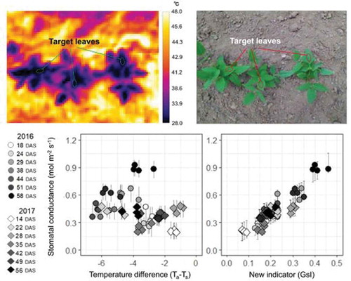
Figure 5. Genetic variability for GsI among 248 accessions of cowpea genetic resources. GsI distributions at vegetative growth stage (a: 5 weeks after sowing) and at the beginning of maturity (b: 8 weeks after sowing). Distribution of the GsI values are separately shown for the three groups of cowpea accessions as per the classification by Fatokun et al. (Citation2018), depending on genomic diversification.
Table 1. Meteorological conditions during measurements in the glasshouse experiment.
Figure 1. Infrared thermal image and RGB image of cowpea plants in the glasshouse experiment (a, b) and in the field experiment (c, d). In the glasshouse experiment, dry and wet references were taken together with the target leaf in a thermal image. In the field experiment, three plants were included in an image and the leaf temperature was detected for the top fully expanded leaves of each plant.
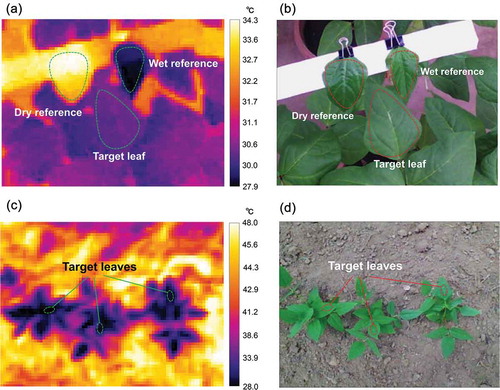
Figure 2. Summary of the regression analysis between stomatal conductance and the thermal indicators in the glasshouse experiment. The relationship (a, c, e) and posterior distributions of the coefficients (b, d, f) are separately shown for each measuring time-point under different meteorological conditions. The regressions between stomatal conductance and GsI (a, b): between stomatal conductance and air-leaf temperature difference (Ta−Ts) (c, d): between stomatal conductance and crop water stress index (CWSI) (e, f). Bar with each point in the scatter plot indicates the 95% interval of the predicted distribution. The box-plots of the coefficients for slope (a) and for constant (b) were generated from 10,000 Markov chain Monte Carlo (MCMC) samples for each measuring time-point.
Figure 3. Meteorological conditions during the field experiment in 2016 and 2017. Weekly average values from 2–8 weeks after sowing are shown for (a) solar radiation, (b) daytime temperature (6:00‒18:00), and (c) daytime vapor pressure deficit (6:00‒18:00). Weekly cumulative values are shown for (d) precipitation.
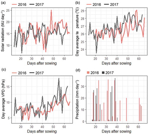
Figure 4. Summary of the regression analysis between stomatal conductance and the thermal indicators in the field experiment. The relationships (a, c) and posterior distributions of the coefficients (b, d) are separately shown for each measuring time-point under different meteorological conditions. Regressions: between stomatal conductance and GsI (a, b): between stomatal conductance and air-leaf temperature difference (Ta−Ts) (c, d). Bars with each point in the scatter plot are the 95% interval of the predicted distribution. The box-plots of the coefficients were generated from 10,000 Markov chain Monte Carlo (MCMC) samples for each time-point.