Method of estimating the lateral vibration of an elevator rope from the vertical vibration of a compensating sheave

Figures & data

Figure 1. Ropes in an elevator shaft. The compensation rope connects the car and the counterweight on the lower side via the compensating sheave for balancing the mass.

Figure 2. Estimation procedure.

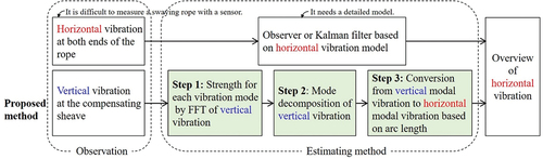
Figure 3. Sinusoidal curve y = a sin x ($0\le x\le \pi$) and its length l. When a straight line of length l bends in the shape of a sin x, the right edge moves to the left by l-π.

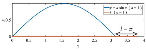
Figure 4. Applicable range of approximate curve. The relation between a and l-π differs depending on whether a is small or large. (a) (0, 0.1]; (b) (0, 10.0].

Table 1. Approximate curves.

Range of a (divided width of a is 0.001)	l-π
0.001 ~ 0.100	0.7835a^2 + 0.0001a
0.001 ~ 1.000	0.6326a^2 + 0.0573a
0.001 ~ 2.000	0.4310a^2 + 0.2356a
0.001 ~ 3.000	0.2993a^2 + 0.4298a

Figure 5. Relation between vertical vibration of the compensating sheave z and horizontal vibration of the compensation rope a.

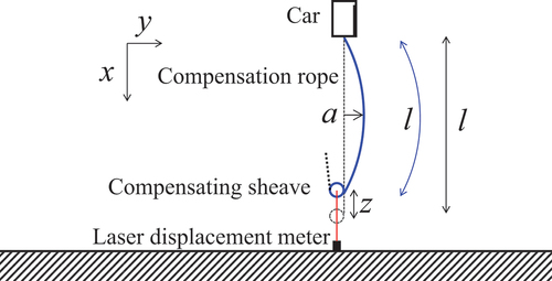
Figure 6. Rope length l when the vertical displacement of the compensating sheave is z and the horizontal amplitude of the compensation rope is a. (b) is the view of (a) from the upper side of the l-axis.

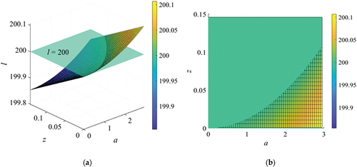
Table 2. Approximate formulae of vertical displacement z. a varies from 0.005 to 2.495 in increments of 0.01. The coefficient of the first-order term increases when the rope length l becomes small.

l	z × 10^3
200	12.3a^2 + 0.0a
175	14.1a^2 + 0.0a
150	16.5a^2 – 0.0a
125	19.7a^2 + 0.0a
100	24.7a^2 – 0.0a
75	32.9a^2 + 0.1a
50	49.5a^2 – 0.1a
25	99.6a^2 – 0.9a

Figure 7. Vertical vibration of the compensating sheave z_N and horizontal vibration of the compensation rope a_N for each mode. (a) 1st; (b) 2nd; (c) 3rd; (d) Combination of 1st to 3rd modes (a₁: a₂: a₃ = 5: 3: 2).

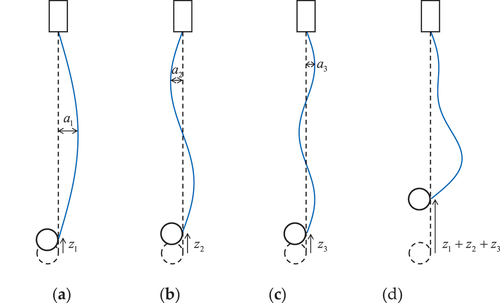
Figure 8. Rope vibration when the tension distribution in the length direction is large.

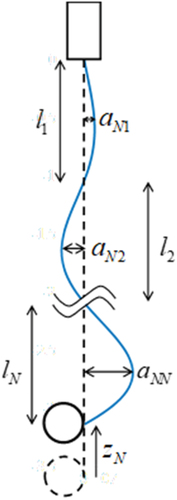
Figure 9. Rope tension distribution and mode shape distortion. (a) Rope tension distribution; (b) mode shape.

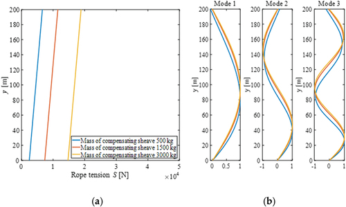
Table 3. Natural frequencies of the building (1st to 5th order).

Mode	1st	2nd	3rd	4th	5th
Natural frequency [Hz]	0.167	0.437	0.708	0.978	1.247

Table 4. Parameters of the analysis model.

Parameter	Symbol	Value
Mass of compensating sheave	–	1500 kg
Mass per unit length of rope	ρ	2.11 kg/m
Damping coefficient per unit length of rope	–	0.0315 N·s/m^2
Length of rope	l	200 m
The number of modes for vibration analysis	Nc	5 ($\ge 3$)
The number of modes for estimation	N0	3
Analysis frequency	Δf	100 Hz
Gravity acceleration	–	9.81 m/s^2
Average tension of rope	$\bar{S}$	$9.4266\times {10}^3$ N
1st natural frequency of rope (Approximate value obtained from average tension)	f1	0.1671 Hz
2nd natural frequency of rope (Approximate value obtained from average tension)	f2	0.3342 Hz
3rd natural frequency of rope (Approximate value obtained from average tension)	f3	0.5013 Hz

Figure 10. Acceleration records resized according to the peak ground velocity of 0.25 m/s, their Fourier amplitude spectra, and displacement disturbance input to the rope. (a) Heisei 16 Niigata Prefecture Chuetsu Earthquake observed in Shinjuku (EW(East-West) component); (b) 2011 Tohoku Earthquake off the Pacific coast observed in Konohana (EW component).

Figure 11. Hamming window for n = 512 (= 2⁹).

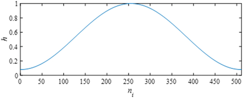
Figure 12. Vertical displacement of the compensating sheave. (a) Heisei 16 Niigata Prefecture Chuetsu Earthquake; (b) 2011 Tohoku Earthquake off the Pacific coast.

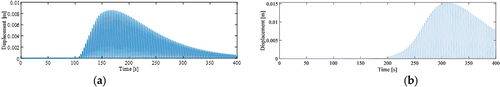
Figure 13. Modal displacements. Five modes are used for numerical analysis, but the responses after the third order are very small. (a) Heisei 16 Niigata Prefecture Chuetsu Earthquake; (b) 2011 Tohoku Earthquake off the Pacific coast.

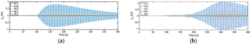
Figure 14. Coefficient of Equation (17)(17) $z_N(t)=\frac{Z(2f_N)}{\sum _{i=1}^{N_0}Z(2f_i)}z(t)\left(N=1,2,\dots ,N_0\right)$(17) (N₀ = 3). The sum of the three values is 1. (a) Heisei 16 Niigata Prefecture Chuetsu Earthquake; (b) 2011 Tohoku Earthquake off the Pacific coast.

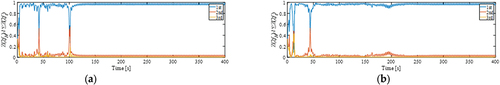
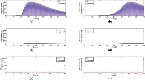
Figure 15. Actual and estimated values of modal responses a_N. (a) 1st mode, (c) 2nd mode, and (e) 3rd mode of the Heisei 16 Niigata Prefecture Chuetsu Earthquake; (b) 1st mode, (d) 2nd mode, and (f) 3rd mode of the 2011 Tohoku Earthquake off the Pacific coast.