Developing simplified numerical calculation and BP neural network modeling for the cooling capacity in a radiant floor cooling system

Figures & data

Table 1. A brief review of floor cooling capacity calculation method.

Reference	Method	Theory principle	Model description for floor construct	Study novelty/Main conclusion
Cholewa et al. (2013)	Experiment	Surface heat flux measurement	Realistic 3D geometry model	Obtained the surface heat transfer coefficients
Pantelic et al. (2018)	Experiment	Surface heat flux measurement	Realistic 3D geometry model	Measured the cooling capacity in the full scale laboratory experiment
Acikgoz et al. (2019)	Experiment	Qt=mw×cp×(Tsp-Tre) Qt=Qr+Qc Qc=hc(Ta-Tf) Qr=hr(AUST-Tf)	Realistic 3D geometry model	Derived the correlations for the convective heat transfer coefficient and total heat flux
Zhu et al. (2022)	Experiment	Qt=mw×cp×(Tsp-Tre) Qt=Qr+Qc Qc=hc(Ta-Tf) Qr=hr(AUST-Tf)	Realistic 3D geometry model	Conducted the experiment on operating characteristic of a combined radiant floor and fan coil cooling system
Zhang et al. (2012)	Analytical solution	Qt=Qr+Qc Qc=hc(Ta-Tf) Qr=hr(AUST-Tf)	Simplified 1D heat transfer model	Obtained a simplified calculation method of cooling/heating capacity and surface temperature distribution of radiant floor
Zhao et al. (2015)	Analytical solution	Qt=Qc+Qlr+Qsr Qc=hc(Ta-Tf) Qr=hr(AUST-Tf)	Simplified 1D heat transfer model	Predicted the cooling capacity of radiant floors in large spaces of an airport
Feng et al. (2016)	Analytical solution	Qt=KΔTh+Qsw_sol	Simplified 1D heat transfer model	Proposed the new simplified method to improve the design of radiant floor with solar radiation.
Tang et al. (2020)	Analytical solution	Qt=A(hc+hlr)(Tz-Tf)	Simplified 1D heat transfer model	Developed the dynamic cooling capacity prediction considering time variable solar radiation
Ren et al. (2021)	Numerical method	$-\mathit{\lambda }\frac{\mathit{\delta T}}{\mathit{\delta x}}=Q_r+Q_c$	Simplified 2D unsteady heat transfer model	Considered the phase change heat transfer process for the phase change energy storage radiant air conditioning system
Fernández-Hernández et al. (2020)	Experiment, numerical method	Qt=Qr+Qc Qc=hc(Ta-Tf) Qr=hr(AUST-Tf)	Simplified 1D heat transfer model	Performed the rotational diffuser coupled with a radiant floor cooling system
Khatri et al. (2020)	Numerical method	N/A	Simplified 1D heat transfer model	Presented the spatial distribution of air temperature and air flow in radiant cooling system
Ning et al. (2022)	RTSM method	$Q_t=\sum _{\mathit{j}=0}^{23}{T}_f(\mathit{n}-\mathit{j})X_f(\mathit{i})\text{break}-\sum _{\mathit{j}=0}^{23}{T}_w(\mathit{n}-\mathit{j})Y_{\mathit{wf}}(\mathit{j})$	Simplified 1D heat transfer model	Concluded the simple and practical advantage of RTSM compared to heat balance method

Note: 1D: one dimensional; 2D: two dimensional; 3D: three dimensional; A: surface area, m²; AUST: the average unheated surface temperature, °C; C_p: water specific heat capacity, J/(kg.K); h_c: convective heat transfer coefficient, W/(m².K); h_lr: longwave radiative heat transfer coefficient, W/(m².K); h_r: radiative heat transfer coefficient, W/(m².K); j: the j^th hour, hour; K_h: the lumped thermal resistance, (m².K)/W; m_w: water supply flow rate, m³/h; n: the current time, hour; RTSM: revised radiant time series method; T_re: water return temperature, °C; T_f: mean floor surface temperature, °C; T_z: the sol–air temperature, °C; T_sp: water supply temperature, °C; T_a: air temperature, °C; Q_t: total heat flux, W/m²; Q_r: radiant heat flux, W/m²; Q_c: convective heat flux, W/m²; Q_lr: longwave radiation flux, W/m²; Q_sr: absorbed shortwave radiation flux, W/m²; X_f: periodic heat absorption response factor, W/(m².K); Y_wf: periodic heat transfer response factor, W/(m².K); λ: conductive heat transfer coefficient, W/(m.K); ΔT_h: mean temperate difference between the cooling medium and space, °C.

Figure 1. Schematic diagram of the three-dimensional computational model: (a) isometric view of the simulation; (b) the pipe arrangement of the floor (Zheng et al. 2017).

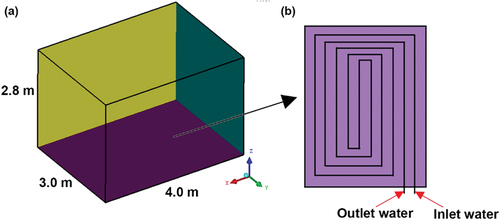
Figure 2. The schematic diagram of a typical radiant floor structure with counterflow water pipes.

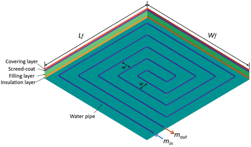
Figure 3. The top view of a simplified counterflow configuration with their dimensions and the pipes’ sequence.

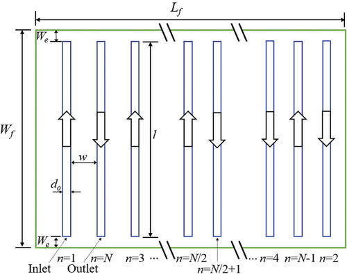
Figure 4. Two configurations of water flow pipes: (a) counterflow; (b) simplified counterflow. Blue sequence numbers indicate the inlet opening, and red sequence numbers indicate the outlet opening.

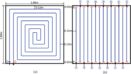
Figure 5. The sectional diagram of a typical radiant floor structure (R20-w200-δ50/20/20).

Table 2. The predefined thickness and thermal physical parameters of the floor structure.

Floor component (Inside to outside)	Thickness (mm)	Density (kg/m^3)	Thermal conductivity (W/m·K)	Specific heat capacity (J/kg·K)
Cover layer	10, 20, 30	2000	0.2, 0.5, 0.8, 1.1, 1.4	950
Screed-coat	20	1700	0.9	1000
Filling layer	40, 50, 60	1800	0.8, 1.0, 1.2, 1.4, 1.6	1000
Pipe	2, 2.5	1050	0.28, 0.33, 0.38, 0.43, 0.48	1000
Insulation	20	400	0.035	2000

Table 3. The descriptions of the pipe length design with different pipe spacings.

Pipe spacing (m)	Distance to the side wall (m)	Total pipe length* (m)	Length per pipe (m)	Total sub-pipe number (-)
0.15	0.16	69.98	3.88	18
0.20	0.16	54.49	3.89	14
0.25	0.125	47.10	3.92	12
0.30	0.15	39.20	3.92	10

Note: * The curvature in the 90-degree bend of the pipe extremities is set as 20 mm.

Table 4. The descriptions of the pipe length design with different floor areas when the pipe spacing is 0.20 m.

Floor surface area, Lf×Wf (m^2)	Total pipe length (m)	Length per pipe (m)
2 × 3	26.62	1.90
3 × 3	4.36	2.88
4 × 3	54.49	3.89
5 × 3	68.44	4.89
6 × 3	82.54	5.90

Table 5. The mean water supply temperature and mass flow rate.

Parameters	Value
Supply water temperature, Tsup (°C)	16, 17, 18, 19, 20
Water mass flow rate, mw (kg/s)	0.03, 0.06, 0.09, 0.12

Table 6. The mixed thermal boundary conditions for the floor surface (Ren et al. 2022; Zhu et al. 2022.).

AUST	External emissivity ε	Indoor air temperature Tair	Heat transfer coefficient hc
29 °C	0.9	26.5 °C	0.87 W/(m^2·K)

Figure 6. The grid distribution in the sectional diagram.

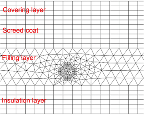
Table 7. The grid independence analysis.

	Pipe element size/Heat source grid size	Total number of grids	ΔT (Floor surface temperature)	ΔT (Air temperature at a height of 1.1 m)
Coarse mesh	1.5 mm/15 m	198,676	-	-
Medium mesh	1 mm/10 mm	291,772	0.73 %	0.94 %
Fine mesh	.8 mm/8 mm	344,672	0.26 %	0.51 %

Note: The boundary layers around the heat source, the grid numbers (≥8) of the inlet and outlet, and the grid number (≥3) for each component in the multilayer structures were kept constant for each case. ΔT means the temperature relative difference.

Figure 7. The schematic diagram of the laboratory: (a) the layout of measurement points; (b) the pipe arrangement in the test room (Acikgoz et al. 2019).

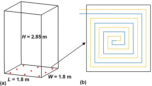
Figure 8. The CFD validation via comparison with the experiment: (a) mean return water temperature; (b) mean floor temperature; (c) total heat transfer flux.

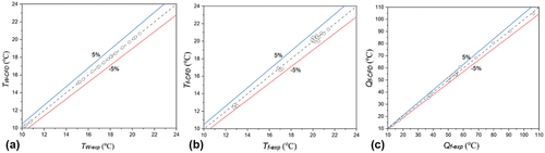
Table 8. The error analysis of the numerical data compared with the experimental data.

	Tw (^oC)	Tf (^oC)	Qt (W/m^2)
Maximum relative error	0.23%	3.56%	5.54%
Average relative error	0.07%	1.24%	2.21%

Figure 9. The structure of the BP neural network (Zhang et al. 2020).

Figure 10. The flow chart of the BP algorithm.

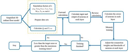
Figure 11. The distribution diagram of the floor temperature (°C) at different sections.

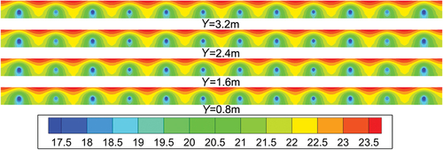
Figure 12. The distribution diagram of the floor temperature (°C) at different values of d_o: (a) d_o = 16 mm; (b) d_o = 20 mm; (c) d_o = 25 mm.

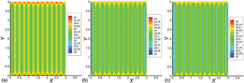
Table 9. The effect of the water supply with and without the pipe wall thickness.

		Tw (^oC)	Tf (^oC)	Qt (W/m^2)
di/do = 12/16 mm	With	19.10	23.82	34.26
	Without	19.18	23.50	36.46
	Relative error (%)	0.38	1.33	6.42
di/do = 16/20 mm	With	19.13	23.72	34.93
	Without	19.19	23.46	36.75
	Relative error (%)	0.28	1.11	5.23
di/do = 20/25 mm	With	19.19	23.51	36.43
	Without	19.26	23.21	38.50
	Relative error (%)	0.35	1.28	5.70

Figure 13. The distribution of Q_t for different floor surface areas.

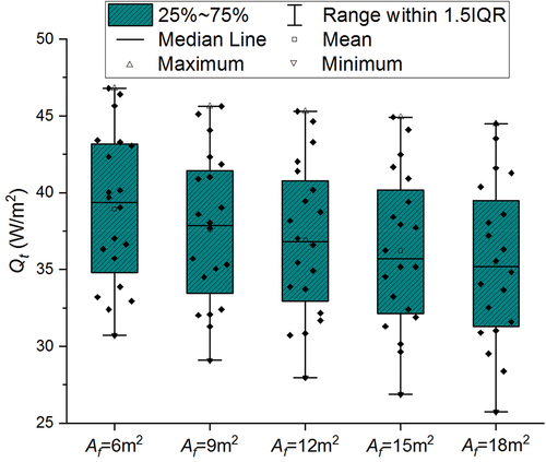
Figure 14. The validation results of the simulated and predicted data: (a, b) the comparison results of the total cooling capacity; (c, d) the comparison results of the minimum temperature.

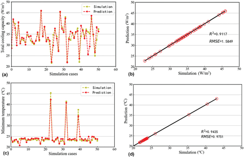
Figure 15. Interfaces of the prediction program: (a) single predict; (b) batch predict; (c) image display.

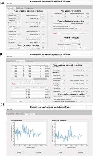
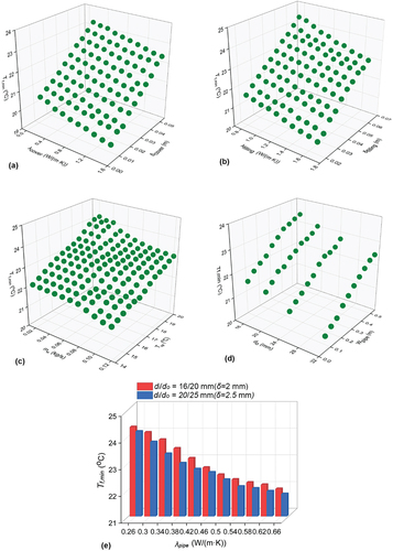
Figure 16. The 3D diagrams of the variation trends of Q_t for different influencing factors: (a) the effects of δ_cover and λ_cover; (b) the effects of δ_filling and λ_filling; (c) the effects of T_sp and m_w; (d) the effects of W_pip and d_o; (e) the effect of λ_pipe.

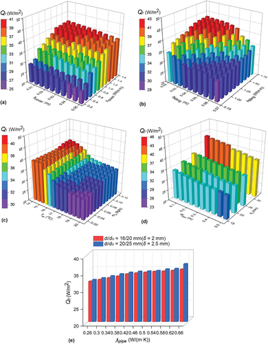
Figure 17. The 3D diagrams of the variation trends of T_f,min for different influencing factors: (a) the effects of δ_cover and λ_cover; (b) the effects of δ_filling and λ_filling; (c) the effects of T_sp and m_w; (d) the effects of W_pip and d_o; (e) the effect of λ_pipe.

Cholewa, T., M. Rosiński, Z. Spik, M. R. Dudzińska, and A. Siuta-Olcha. 2013. “On the Heat Transfer Coefficients Between Heated/Cooled Radiant Floor and Room.” Energy and Buildings 66:599–606. https://doi.org/10.1016/j.enbuild.2013.07.065.

 Web of Science ®Google Scholar

Pantelic, J., S. Schiavon, B. Ning, E. Burdakis, P. Raftery, and F. Bauman. 2018. “Full Scale Laboratory Experiment on the Cooling Capacity of a Radiant Floor System.” Energy and Buildings 170:134–144. https://doi.org/10.1016/j.enbuild.2018.03.002.

 Web of Science ®Google Scholar

Acikgoz, O., Y. Karakoyun, Z. Yumurtacı, N. Dukhan, and A. S. Dalkılıç. 2019. “Realistic Experimental Heat Transfer Characteristics of Radiant Floor Heating Using Sidewalls as Heat Sinks.” Energy and Buildings 183:515–526. https://doi.org/10.1016/j.enbuild.2018.11.022.

 Web of Science ®Google Scholar

Zhu, X., J. Liu, X. Zhu, X. Wang, Y. Du, and J. Miao. 2022. “Experimental Study on Operating Characteristic of a Combined Radiant Floor and Fan Coil Cooling System in a High Humidity Environment.” Buildings 12 (4): 499. https://doi.org/10.3390/buildings12040499.

 Web of Science ®Google Scholar

Zhang, L., X.-H. Liu, and Y. Jiang. 2012. “Simplified Calculation for Cooling/Heating Capacity, Surface Temperature Distribution of Radiant Floor.” Energy and Buildings 55:397–404. https://doi.org/10.1016/j.enbuild.2012.08.026.

 Web of Science ®Google Scholar

Zhao, K., X.-H. Liu, and Y. Jiang. 2015. “Cooling Capacity Prediction of Radiant Floors in Large Spaces of an Airport.” Solar Energy 113:221–235. https://doi.org/10.1016/j.solener.2015.01.003.

 Web of Science ®Google Scholar

Feng, J., S. Schiavon, and F. Bauman. 2016. “New Method for the Design of Radiant Floor Cooling Systems with Solar Radiation.” Energy and Buildings 125:9–18. https://doi.org/10.1016/j.enbuild.2016.04.048.

 Web of Science ®Google Scholar

Tang, H., T. Zhang, X. Liu, and C. Li. 2020. “A Novel Approximate Harmonic Method for the Dynamic Cooling Capacity Prediction of Radiant Slab Floors with Time Variable Solar Radiation.” Energy and Buildings 223:110117. https://doi.org/10.1016/j.enbuild.2020.110117.

 Web of Science ®Google Scholar

Ren, F., J. Du, Y. Cai, Z. Xu, D. Zhang, and Y. Liu. 2021. “Numerical Simulation Study on Thermal Performance of Sub-Tropical Double-Layer Energy Storage Floor Combined with Ceiling Energy Storage Radiant Air Conditioning.” Case Studies in Thermal Engineering 28:101696. https://doi.org/10.1016/j.csite.2021.101696.

 Web of Science ®Google Scholar

Fernández-Hernández, F., A. Fernández-Gutiérrez, J. J. Martínez-Almansa, C. Del Pino, and L. Parras. 2020. “Flow Patterns and Heat Transfer Coefficients Using a Rotational Diffuser Coupled with a Radiant Floor Cooling.” Applied Thermal Engineering 168:114827. https://doi.org/10.1016/j.applthermaleng.2019.114827.

 Web of Science ®Google Scholar

Khatri, R., V. R. Khare, and H. Kumar. 2020. “Spatial Distribution of Air Temperature and Air Flow Analysis in Radiant Cooling System Using CFD Technique.” Energy Reports 6:268–275. https://doi.org/10.1016/j.egyr.2019.11.073.

 Web of Science ®Google Scholar

Ning, B., M. Zhang, J. Li, and Y. Chen. 2022. “A Revised Radiant Time Series Method (RTSM) to Calculate the Cooling Load for Pipe-Embedded Radiant Systems.” Energy and Buildings 268:112199. https://doi.org/10.1016/j.enbuild.2022.112199.

 Web of Science ®Google Scholar

Zheng, X., Y. Han, H. Zhang, W. Zheng, and D. Kong. 2017. “Numerical Study on Impact of Non-Heating Surface Temperature on the Heat Output of Radiant Floor Heating System.” Energy and Buildings 155:198–206. https://doi.org/10.1016/j.enbuild.2017.09.022.

 Web of Science ®Google Scholar

Ren, J., J. Liu, S. Zhou, M. K. Kim, and S. Song. 2022. “Experimental Study on Control Strategies of Radiant Floor Cooling System with Direct-Ground Cooling Source and Displacement Ventilation System: A Case Study in an Office Building.” Energy 239:122410. https://doi.org/10.1016/j.energy.2021.122410.

 Web of Science ®Google Scholar

Zhang, T., Y. Liu, Y. Rao, X. Li, and Q. Zhao. 2020. “Optimal Design of Building Environment with Hybrid Genetic Algorithm, Artificial Neural Network, Multivariate Regression Analysis and Fuzzy Logic Controller.” Building & Environment 175:106810. https://doi.org/10.1016/j.buildenv.2020.106810.

 Web of Science ®Google Scholar