Spatiotemporal evolution of carbon emissions and influencing factors in county-level based on nighttime lighting data: a case study in Huaihai economic zone core city

Figures & data

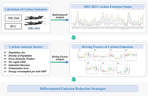
Figure 1. 57 Districts and Counties in the Huaihai economic zone core city cluster study area. The scope of the study area follows the hierarchical relationship of provincial, city, and county levels from large to small. Figure a shows the spatial location of the Huaihai economic zone in China and its provincial relationships with the four surrounding provinces; figure b shows the extent of the city-level areas and core cities included in the Huaihai economic zone; and figure c shows the 57 county-level areas included in the core cities of the Huaihai economic zone.

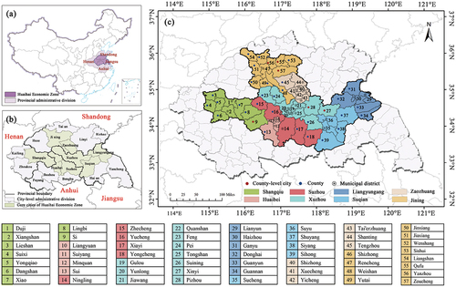
Table 1. Verification of spatial autocorrelation.

Data Name	Data Description	Source
Nighttime light	DMSP/OLS nighttime light	National Oceanic and Atmospheric Administration’s National Geophysical Data Center (NOAA/NGDC)
	NPP/VIIRS nighttime light	Colorado School of Mines
Fossil fuel combustion data	Annual total data of ten energy types, such as raw coal, coke, crude oil, gasoline, kerosene, diesel oil, fuel oil, natural gas, heat and electricity, during 2001–2021	China Statistical Yearbook, China Regional Statistical Yearbook, China Energy Statistical Yearbook and statistical yearbooks of each city
Socioeconomic data	Annual statistical data of six types, such as permanent population, GDP, per capita GDP, primary industry GDP, secondary industry GDP and tertiary industry GDP, during 2001–2021	China Statistical Yearbook, China City Statistical Yearbook, China Regional Statistical Yearbook, and statistical yearbooks of each city
Administrative boundaries	Vector files of provinces, prefectures in China	National Catalogue Service For Geographic Information
Population density	Annual data with a spatial resolution of 30 arc-seconds (approximately 1km at the equator)	OpenStreetMap (https://download.geofabrik.de/asia/china.html. accessed 3 December 2022)

Figure 2. Technical roadmap.

Figure 3. Nighttime lighting data in Huaihai economic zone core city in 2001 (a) and 2021 (b).

Table 2. Energy carbon emission factors.

Energy Type	Conversion Standard Coal Coefficient (tons of standard coal/ton)	Carbon Emission Coefficient (10^4 tons carbon/10^4 tons standard coal)
Raw Coal	0.7143	0.7559
Coke	0.9714	0.855
Crude Oil	1.4286	0.5857
Gasoline	1.4714	0.5538
Kerosene	1.4714	0.5714
Diesel	1.4751	0.5921
Fuel Oil	1.4286	0.6185
Natural Gas	1.33	0.4483
Heat	34.12	0.67
Electricity	0.345	0.272

Table 3. County carbon dioxide emissions in a linear regression model using data on evening light levels in a grayscale format.

Year	A	$R^2$	Year	A	$R^2$
2001	0.0005	0.9014	2012	0.0006	0.9402
2002	0.0006	0.9046	2013	0.0007	0.9498
2003	0.0005	0.9008	2014	0.0013	0.9526
2004	0.0007	0.9065	2015	0.0008	0.9507
2005	0.0006	0.9253	2016	0.0006	0.9524
2006	0.0005	0.9476	2017	0.0004	0.9643
2007	0.0007	0.9574	2018	0.0005	0.9265
2008	0.0006	0.9648	2019	0.0004	0.9671
2009	0.0007	0.9504	2020	0.0004	0.9687
2010	0.0005	0.9434	2021	0.0003	0.9752
2011	0.0005	0.9456

Figure 4. Scatter plot of IPCC statistical CO₂ emission values versus fitted CO₂ emission values.

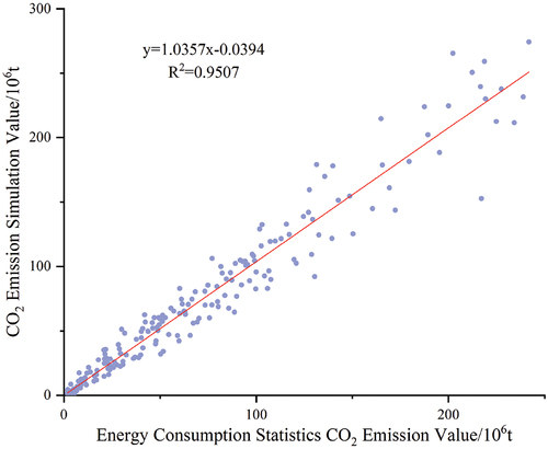
Table 4. Spatial autocorrelation verification.

$\mathit{Z}$Score	$\mathit{P}$Value	Spatial Autocorrelation
$\mathit{Z}$≤ 1.96	$\mathit{P}$> 0.05	Non-existent
$\mathit{Z}$≥ 1.96	$\mathit{P}$< 0.05	Exist
$\mathit{Z}$≥ 2.58	$\mathit{P}$< 0.01	Extremely strong

Table 5. Definition of carbon emission impact factors indicators.

Variable Dimension		Abbreviations	Explanatory variables	Unit
F1	Population size	POP	Total household population by county	million people
F2	Density of Population	DOP	Number of people per unit of land area	People /km^2
F3	Gross Domestic Product	GDP	Gross regional product by county	million RMB
F4	Per capita GDP	PGDP	GDP per capita	million RMB
F5	Industrial Structure	SIND	The scale of output value of secondary industry	million RMB
F6	Urbanization level	UR	Non-agricultural population as a proportion of the total regional population	%
F7	Energy consumption per unit GDP	EI	Energy consumption per unit of GDP	Tons/RMB

Table 6. Statistical description of relevant variables.

Variables	F1	F2	F3	F4	F5	F6	F7
Mean value	83.78	907.92	155.57	2.03	44.167	36.48	2.92
Standard deviation	45.33	1090.54	179.78	1.04	11.66	23.63	2.09
Minimum value	13.14	255.47	8.27	0.26	9.97	6.46	0.26
Maximum Value	439.87	8299.83	1085.37	2.03	81.64	99.98	14.53

Figure 5. Trends of total carbon emissions in core cities and counties of the Huaihai economic zone, 2001–2021.

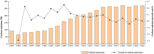
Figure 6. Changes in carbon emissions by district and counties,2001–2021.

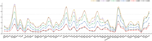
Figure 7. (a) State of carbon emission in the Huaihai economic zone in 2001, (b) state of carbon emission in the Huaihai economic zone in 2005, (c) state of carbon emission in the Huaihai economic zone in 2009, (d) state of carbon emission in the Huaihai economic zone in 2013, (e) state of carbon emission in the Huaihai economic zone in 2017, (f) state of carbon emission in the Huaihai economic zone in 2021; spatial and temporal changes in carbon emissions 2001–2021.

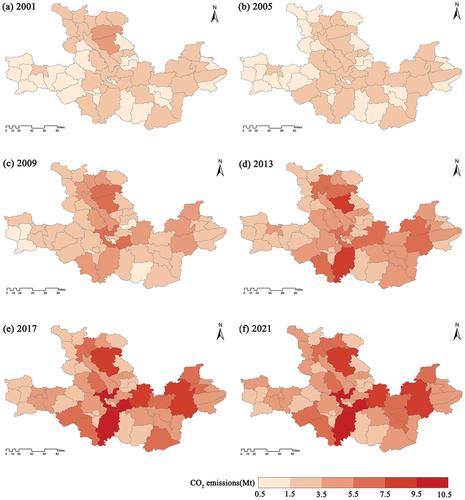
Table 7. Global Moran’s I of CO₂ emissions at the county level, 2001– 2021.

Year	Global Moran’s I	Z Score	P Value
2001	0.5235	4.8508	0.001
2002	0.5264	5.1121	0.001
2003	0.4206	4.0567	0.001
2004	0.4632	4.3368	0.001
2005	0.4065	4.1276	0.001
2006	0.3955	3.8757	0.003
2007	0.3921	3.7671	0.002
2008	0.4018	3.9795	0.001
2009	0.4555	4.3931	0.001
2010	0.4422	4.2318	0.001
2011	0.4522	4.3683	0.001
2012	0.4547	4.3911	0.001
2013	0.4451	4.3295	0.001
2014	0.4366	4.0091	0.001
2015	0.4155	3.8521	0.001
2016	0.4116	3.9886	0.001
2017	0.4061	4.0993	0.001
2018	0.4063	4.2453	0.001
2019	0.4065	4.1419	0.001
2020	0.4016	4.0977	0.001
2021	0.3914	3.8957	0.002

Figure 8. Spatial autocorrelation local clustering analysis of carbon emissions. (a) Carbon emission local cluster analysis, 2001. (b) Carbon emission local cluster analysis, 2005. (c) Carbon emission local cluster analysis, 2009. (d) Carbon emission local cluster analysis, 2013. (e) Carbon emission local cluster analysis, 2017. (f) Carbon emission local cluster analysis, 2021.

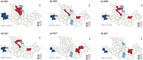
Figure 9. Spatial autocorrelation local significance analysis of carbon emissions. (a) Carbon emission local significance analysis, 2001. (b) Carbon emission local significance analysis, 2005. (c) Carbon emission local significance analysis, 2009. (d) Carbon emission local significance Analysis, 2013. (e) Carbon emission local significance analysis, 2017. (b) Carbon emission local significance analysis, 2021.

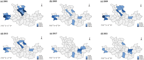
Table 8. Multi-collinearity test.

Variables	F1	F2	F3	F4	F5	F6	F7
Tolerance	0.508	0.658	0.415	0.554	0.859	0.505	0.537
VIF	1.969	1.519	2.409	1.806	1.165	1.979	1.864

Table 9. Comparison of model evaluation indexes.

Variables	OLS	GTWR
AIC	1032.01	802.383
R^2	0.7122	0.9346
Adjustment of R^2	0.7014	0.9332
AIC change amount	0	229.627
R^2 change amount	0	0.2224

Table 10. Descriptive statistics of regression coefficients of the GTWR model.

Variables		Minimum	Maximum	Average	Median	Standard deviation
F1	POP	−0.0136	1.7414	0.7193	0.3742	0.6577
F2	DOP	−0.6713	0.4024	−0.0428	0.0135	0.1749
F3	GDP	0.2149	7.3182	3.0153	3.3582	2.4939
F4	PGDP	−0.2165	0.9589	0.3298	0.2704	0.3054
F5	SIND	−0.1320	−0.5325	0.0951	0.0129	0.1944
F6	UR	−0.2410	0.5267	0.0059	−0.0771	0.1951
F7	EI	0.4675	2.6747	0.8681	0.7068	0.4614

Figure 10. Time series change trend of GTWR regression coefficients. (a) F1 (POP) time series trends of regression coefficients, 2001–2021; (b) F2 (DOP) time series trends of regression coefficients, 2001–2021; (c) F3(GOP)Time series trends of regression coefficients, 2001–2021; (d) F4(PGOP) time series trends of regression coefficients, 2001–2021; (e) F5 (SIJND) time series trends of regression coefficients, 2001–2021; (f) F6(UR)time series trends of regression coefficients, 2001–2021; (g) F7(UR)Time series trends of regression coefficients, 2001–2021.

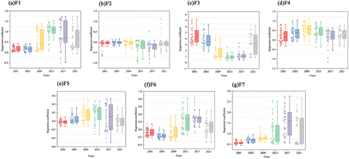
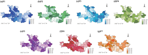
Figure 11. Spatial distribution patterns of carbon emission influencing factors based on GTWR model. (a) F1(POP)Spatial distribution characteristics of county territory. (b) F2(DOP)Spatial distribution characteristics of county territory. (c) F3(GOP)Spatial distribution characteristics of county territory. (d) F4 (Pgop)spatial distribution characteristics of county territory. (e) F5(SIJND)Spatial distribution characteristics of county territory. (f) F6(UR)Spatial distribution characteristics of county territory. (g) F7(EI) spatial distribution characteristics of county territory.