Similarities in face and voice cerebral processing

Figures & data

Figure 1. Temporal Voice Areas (TVAs) in the human brain. A cluster analysis of the density map of voice > nonvoice contrast revealing three main clusters of voice sensitivity in each hemisphere along a voice-sensitive zone of cortex extending from posterior STS to mid-STS/STG to anterior STG. The cluster with the greatest peak density is in right pSTS, consistent with individual images. Reproduced (permission pending) from Pernet et al. (2015).

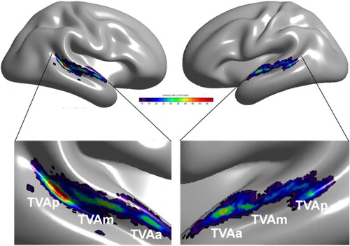
Figure 2. Norm-based coding of speaker identity in the Temporal Voice Areas. (A) TVA showing significantly greater fMRI signal in response to vocal versus nonvocal sounds at the group-level used as a mask for further analysis. Colour scale indicates T values of the vocal versus nonvocal contrast. (B) Maps of Spearman correlation between beta estimates of BOLD signal in response to each voice stimulus and its distance-to-mean overlay on the TVA map (black). Colour scale indicates significant r values (p < .05 corrected for multiple comparisons). Note a bilateral distribution with a maximum along the right anterior STS. (C) Scatterplots and regression lines between estimates of BOLD signal and distance-to-mean at the peak voxel for “had” syllables. (D) Scatterplots and regression lines between estimates of BOLD signal and distance-to-mean at the peak voxel observed for “hellos”. Reproduced (permission pending) from Latinus et al. (2013).

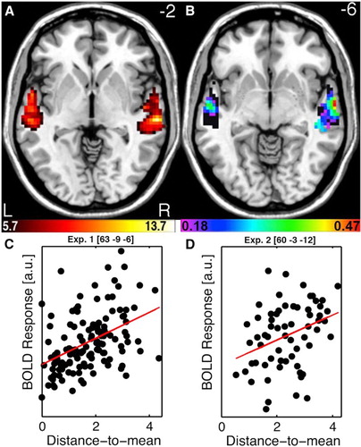
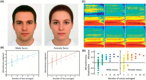
Figure 3. Averaging and attractiveness in faces and voices. Face and voice attractiveness judgments as a function of averaging. (A) Face composites generated by averaging 32 male faces (left) and 64 female faces (right). (B) Attractiveness ratings as a function of number of face averaged. Note the steady increase in attractiveness ratings with increasing number of averaged faces, for both male (left) and female (right) faces. Reproduced, with permission, from Braun, Gruendl, Marberger, and Scherber (2001). (C) Spectrograms of voice composites generated by averaging an increasing number of voices of the same gender (different speakers uttering the syllable “had”). (D) Attractiveness ratings as a function of number of voices averaged. Note the steady increase in attractiveness ratings with increasing number of averaged voices, for both male (left) and female (right) voices. Reproduced (permission pending) from Bruckert et al. (2010).

Pernet, C. R., McAleer, P., Latinus, M., Gorgolewski, K. J., Charest, I., Bestelmeyer, P. E., …  Belin, P. (2015). The human voice areas: Spatial organization and inter-individual variability in temporal and extra-temporal cortices. NEUROIMAGE, 119, 164–174. doi: 10.1016/j.neuroimage.2015.06.050

 PubMed Web of Science ®Google Scholar

Latinus, M., McAleer, P., Bestelmeyer, P. E., & Belin, P. (2013). Norm-based coding of voice identity in human auditory cortex. Current Biology, 23(12), 1075–1080. doi: 10.1016/j.cub.2013.04.055

 PubMed Web of Science ®Google Scholar

Braun, C., Gruendl, M., Marberger, C., & Scherber, C. (2001). Beautycheck - Ursachen und Folgen von Attraktivitae.

 Google Scholar

Bruckert, L., Bestelmeyer, P., Latinus, M., Rouger, J., Charest, I., Rousselet, G. A., … Belin, P. (2010). Vocal attractiveness increases by averaging. Current Biology, 20(2), 116–120. doi: 10.1016/j.cub.2009.11.034

 PubMed Web of Science ®Google Scholar