On the statistics of scaling exponents and the multiscaling value at risk

Figures & data

Figure 1. ACSR methodology computed on the autocorrelation function of the absolute values of the log-returns time series. The red circle shows the breakpoint where the regression line has a break.

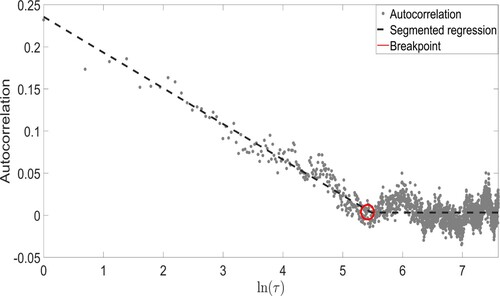
Table 1. Results of the ACSR for the estimation of ${\tau }_{max}$. ${\overline{\tau }}^{\ast }$ is the mean over all the paths and the $95\mathrm{\%}$ C.I. are computed over 200,000 bootstrapped samples.

	${\overline{\tau }}^{\ast }$	95% C.I.
$\lambda =0.05$	297.2	(239.8,354.7)
$\lambda =0.10$	267.8	(243.2,292.4)
$\lambda =0.30$	259.9	(231.6,288.3)

Table 2. RMSE for the parameter A for the different methodologies.

	GHE	RNSGHEL	NSGHENL	RNSGHENL
$\lambda =0.05$	0.0338	0.0148	0.0163	0.0163
$\lambda =0.10$	0.0289	0.0147	0.0154	0.0153
$\lambda =0.30$	0.0427	0.0352	0.0343	0.0339

Note: Subscript L refers to the linear regression while NL to the non-linear regression.

Table 3. RMSE for the parameter B for the different methodologies.

	GHE	RNSGHEL	NSGHENL	RNSGHENL
$\lambda =0.05$	0.0112	0.0039	0.0047	0.0039
$\lambda =0.10$	0.0098	0.0043	0.0046	0.0043
$\lambda =0.30$	0.0167	0.0144	0.0137	0.0144

Note: Subscript L refers to the linear regression while NL to the non-linear regression.

Figure 2. p-Values of all the 50 coefficients related to q moments equations for a multifractal random walk with T = 10, 000, $\lambda =0.05$, L = 250 and $\sigma =1$.

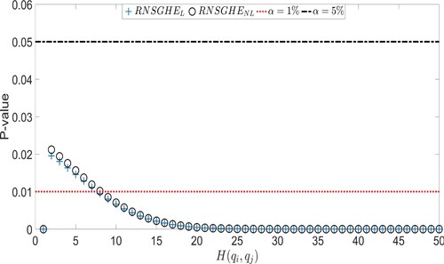
Table 4. p-Values of the F-test for the null that only $H(0,q_1)$ is different from 0.

	RNSGHEL	RNSGHENL
$\lambda =0.05$	0.99999	0.99999
$\lambda =0.10$	0.00003	0.00003
$\lambda =0.30$	0.00000	0.00000

Note: Subscript L refers to linear regression while NL to non-linear regression.

Table 5. Summary statistics of the log-returns of the analyzed stocks.

	Summary statistics
Stock	Mean	Median	Min	Max	Std	Skewness	Kurtosis	Obs
AAPL	0.00	0.00	−0.73	0.13	0.03	−4.08	115.62	5362
AXP	0.00	0.00	−0.19	0.19	0.02	−0.05	13.72	5362
BA	0.00	0.00	−0.19	0.14	0.02	−0.27	8.72	5362
CAT	0.00	0.00	−0.16	0.14	0.02	−0.16	7.59	5362
CSCO	0.00	0.00	−0.17	0.22	0.02	0.14	12.31	5362
CVX	0.00	0.00	−0.13	0.19	0.02	0.07	13.68	5362
DIS	0.00	0.00	−0.20	0.15	0.02	−0.10	14.05	5362
GS	0.00	0.00	−0.21	0.28	0.02	0.61	18.47	5362
HD	0.00	0.00	−0.34	0.13	0.02	−0.98	26.78	5362
IBM	0.00	0.00	−0.21	0.12	0.02	−0.43	15.84	5362
INTC	0.00	0.00	−0.25	0.18	0.02	−0.44	11.89	5362
JN'	0.00	0.00	−0.17	0.12	0.01	−0.61	18.33	5362
JPM	0.00	0.00	−0.23	0.22	0.02	0.25	17.55	5362
KO	0.00	0.00	−0.11	0.13	0.01	0.05	12.27	5362
MCD	0.00	0.00	−0.14	0.09	0.01	−0.09	9.97	5362
MMM	0.00	0.00	−0.14	0.10	0.01	−0.20	9.69	5362
MRK	0.00	0.00	−0.31	0.12	0.02	−1.36	31.86	5362
MSFT	0.00	0.00	−0.17	0.18	0.02	−0.09	12.65	5362
NKE	0.00	0.00	−0.22	0.18	0.02	−0.18	15.88	5362
PFE	0.00	0.00	−0.12	0.10	0.02	−0.27	8.59	5362
PG	0.00	0.00	−0.38	0.10	0.01	−4.21	120.73	5362
TRV	0.00	0.00	−0.20	0.23	0.02	0.31	19.69	5362
UNH	0.00	0.00	−0.22	0.30	0.02	0.05	23.74	5362
UTX	0.00	0.00	−0.33	0.13	0.02	−1.44	36.30	5362
VZ	0.00	0.00	−0.13	0.14	0.01	0.13	9.89	5362
WMT	0.00	0.00	−0.11	0.11	0.01	0.21	10.11	5362
XOM	0.00	0.00	−0.15	0.16	0.01	0.05	13.43	5362

Table 6. Results of the multiscaling estimation and testing procedure.

Stock	${\tau }^{\mathbf{\ast }}$	Weak M-S	Strong M-S	RW t-test	M-S F-test	$\hat{H}$	$\hat{A}$	$\hat{B}$
AAPL	963	NO	YES	NO	YES	0.5567	0.5774	−0.0407
						(0.5534, 0.5600)	(0.5770, 0.5779)	(−0.0414, −0.0399)
AXP	1072	NO	YES	NO	YES	0.5203	0.5535	−0.0653
						(0.5149, 0.5256)	(0.5525, 0.5545)	(−0.0670, −0.0636)
BA	1072	NO	YES	NO	YES	0.5391	0.5630	−0.0468
						(0.5353, 0.5429)	(0.5623, 0.5637)	(−0.0480, −0.0456)
CAT	527	NO	YES	NO	YES	0.5422	0.5603	−0.0355
						(0.5393, 0.5451)	(0.5597, 0.5608)	(−0.0364, −0.0345)
CSCO	1072	NO	YES	YES	YES	0.5011	0.5292	−0.0551
						(0.4966, 0.5056)	(0.5280, 0.5304)	(−0.0571, −0.0530)
CVX	313	NO	YES	NO	YES	0.4722	0.4872	−0.0293
						(0.4699, 0.4746)	(0.4868, 0.4876)	(−0.0300, −0.0286)
DIS	1072	NO	YES	NO	YES	0.5211	0.5410	−0.0389
						(0.5180, 0.5243)	(0.5406, 0.5413)	(−0.0395, −0.0382)
GS	1070	NO	YES	NO	YES	0.4861	0.5110	−0.0489
						(0.4821, 0.4901)	(0.5102, 0.5118)	(−0.0503, −0.0475)
HD	1072	NO	YES	NO	YES	0.5370	0.5614	−0.0477
						(0.5332, 0.5409)	(0.5608, 0.5619 )	(−0.0486, −0.0467)
IBM	1072	NO	YES	NO	YES	0.4842	0.5053	−0.0413
						(0.4808, 0.4876)	(0.5049, 0.5057)	(−0.0420, −0.0407)
INTC	1072	NO	YES	NO	YES	0.4568	0.4797	−0.0450
						(0.4531, 0.4605)	(0.4786, 0.4809)	(−0.0470, −0.0430)
JN	488	NO	YES	NO	YES	0.4664	0.4880	−0.0423
						(0.4629, 0.4698)	(0.4874, 0.4885 )	(−0.0432, −0.0415)
JPM	1072	NO	YES	NO	YES	0.4851	0.5124	−0.0535
						(0.4808, 0.4895)	(0.5118, 0.5131)	(−0.0546, −0.0523)
KO	1072	NO	YES	NO	YES	0.4937	0.5134	−0.0387
						(0.4905, 0.4968)	(0.5129, 0.5139)	(−0.0395, −0.0379)
MCD	480	NO	YES	NO	YES	0.5116	0.5266	−0.0293
						0.5092, 0.5140)	(0.5261, 0.5270)	(−0.0301, −0.0286)
MMM	1032	NO	YES	NO	YES	0.4564	0.4747	−0.0360
						(0.4534, 0.4593)	(0.4743, 0.4751)	(−0.0366, −0.0353)
MRK	867	NO	YES	NO	YES	0.5231	0.5498	−0.0522
						(0.5189, 0.5274)	(0.5484, 0.5512)	(−0.0546, −0.0499)
MSFT	1072	NO	YES	NO	YES	0.4737	0.4981	−0.0479
						(0.4698, 0.4776)	(0.4975, 0.4988)	(−0.0490, −0.0468)
NKE	1072	NO	YES	NO	YES	0.4763	0.4913	−0.0295
						(0.4739, 0.4787 )	(0.4912, 0.4915)	(−0.0298, −0.0292)
PFE	1072	NO	YES	YES	YES	0.4999	0.5285	−0.0562
						(0.4952, 0.5046)	(0.5263, 0.5308)	(−0.0600, −0.0523)
PG	969	NO	YES	NO	YES	0.4617	0.4834	−0.0426
						(0.4582, 0.4652)	(0.4829, 0.4839)	(−0.0435, −0.0417)
TRV	604	NO	YES	NO	YES	0.4673	0.4861	−0.0368
						(0.4643, 0.4703)	(0.4857, 0.4865)	(−0.0375, −0.0362)
UNH	580	NO	YES	NO	YES	0.5163	0.5346	−0.0360
						(0.5134, 0.5192)	(0.5342, 0.5351)	(−0.0367, −0.0352)
UTX	1072	NO	YES	NO	YES	0.4799	0.5053	−0.0497
						(0.4759, 0.4840)	(0.5048, 0.5059)	(−0.0507, −0.0488)
VZ	1072	NO	YES	NO	YES	0.4712	0.4897	−0.0362
						(0.4683, 0.4742)	(0.4889, 0.4905)	(−0.0376, −0.0348)
WMT	1072	NO	YES	NO	YES	0.4314	0.4540	−0.0444
						(0.4277, 0.4350)	(0.4534, 0.4546)	(−0.0454, −0.0434)
XOM	344	NO	YES	NO	YES	0.4642	0.4852	−0.0413
						(0.4608, 0.4675)	(0.4846, 0.4858)	(−0.0422, −0.0403)

Figure 3. Verizon log-prices time series and some anomalies of financial time series.

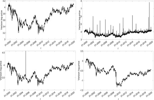
Figure 4. Cumulative Variance (CV) and Cumulative Auto-Covariance (CAV) for the Verizon time series.

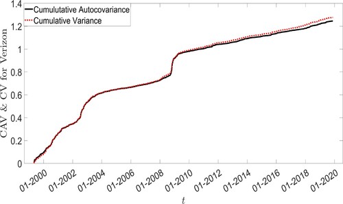
Figure 5. Cumulative Variance ($CV(t)$) and Cumulative Auto-Covariance ($CAV(t)$) for the Verizon time series (top panel) and the measure $D(t)$ (bottom panel) in case of the added spike.

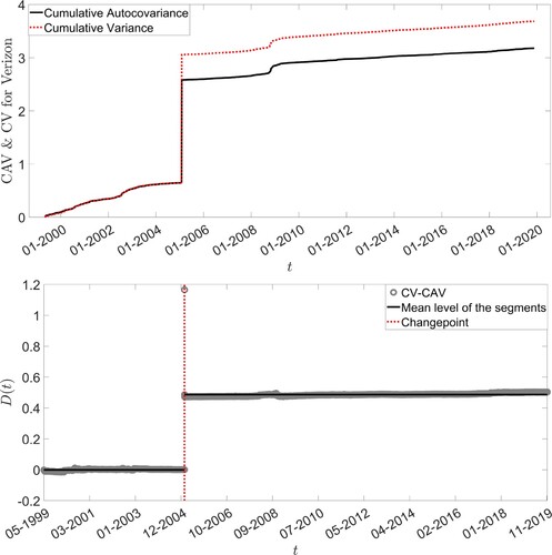
Figure 6. Cumulative Variance ($CV(t)$) and Cumulative Auto-Covariance ($CAV(t)$) for the Verizon time series (top panel) and the measure $D(t)$ (bottom panel) in case of the added jump.

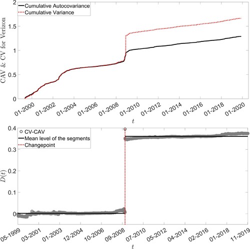
Table 7. Results of the multiscaling estimation on the times series reported in Figure 3 (bottom panels) with anomalies not removed.

	$\hat{H}$	$\hat{A}$	$\hat{B}$
Spike	0.5290	0.6013	−0.1417
Jump	0.4942	0.5220	−0.0543

Table 8. Average of the 100 estimated $\hat{H}$, $\hat{A}$ and $\hat{B}$ for a fractional Brownian motion with H = 0.47. $95\mathrm{\%}$ C.I. computed over 200,000 bootstrapped samples are reported in parenthesis.

	$\hat{H}$	$\hat{A}$	$\hat{B}$
No anomalies	0.4663 (0.4597, 0.4710)	0.4654 (0.4596, 0.4728)	−0.0018 (−0.0048, 0.0012)
Spike	0.4403 (0.4330, 0.4481)	0.4893 (0.4799, 0.4998)	−0.0961 (−0.1027, −0.0899)
Jump	0.4845 (0.4785, 0.4905)	0.4806 (0.4737, 0.4874)	0.0076 (0.0045, 0.011)

Table 9. Results of the jump detection analysis and estimated exponent parameters.

	Jump date	$\hat{H}$	$\hat{A}$	$\hat{B}$
AAPL	29 September 2000	0.5315	0.5527	−0.0416
HD	12 October 2000	0.5203	0.5535	−0.0653
MRK	30 September 2004	0.5391	0.5630	−0.0468
PG	7 March 2000	0.5422	0.5603	−0.0355
UNH	13 October 2008	0.5011	0.5292	−0.0551
UTX	17 September 2001	0.4722	0.4872	−0.0293

Figure 7. HVaR using annual data and using daily data rescaled by the factor ${250}^{0.5}$ and by ${250}^{\hat{H}}$. Stocks are sorted by the magnitude of the annual Historical VaR.

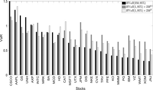
Figure 8. GVaR using annual data and using daily data rescaled by the factor ${250}^{0.5}$ and by ${250}^{\hat{H}}$. Stocks are sorted by the magnitude of the annual Gaussian VaR.

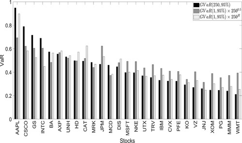
Figure 9. Relative error between the true VaR calculated using annual data, HVaR and GVaR computed using daily data scaled by the factor 0.5 and by the estimated factor H. The red line is the 45 degrees reference line.

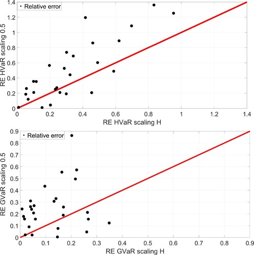
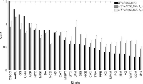
Figure 10. Annual Historical VaR (HVaR) and Multiscaling VaR (MSVaR). Confidence level $95\mathrm{\%}$. Stocks are sorted according to the magnitude of the Historical VaR.