Analysing emerging market returns with high-frequency data during the global financial crisis of 2007–2009

Figures & data

Table 1. Transaction hours for Borsa Istanbul.

Issue date and number	Date of validity	Changes that made	Continuous trading method session hours
06/08/2001 (151)	13.08.2001	It was determined as 09:30 - 12:00 (First Session) and 14:00 - 16:30 (Second Session). “Order Submission with Floppy” times have been re-determined as 09:30 - 10:00 for the first session and as 14:00 - 14:15 for the second session.	First session: 09:30 - 12:00Second session: 14:00 - 16:30
27/11/2006 (255)	2.02.2007	Opening session	Opening session: 09:30 - 09:50 - 10:00First session: 10:00 - 12:00Second session: 14:00 - 16:30
06/08/2007 (267)	7.09.2007	The end of the second session was moved from 16:30 to 17:00.	Opening session: 09:30 - 09:40 - 09:45First session: 09:45 - 12:00Second session: 14:00 - 17:00
08/09/2008 (288)	13.10.2008	The first session opening was increased to 15 + 5 by removing the floppy disk and the end of the first session was made at 12:30.	Opening session: 09:30 - 09:45 - 09:50First session: 09:50 - 12:30Second session: 14:00 - 17:00
14/09/2009 (306)	19.10.2009	The end of the second session was moved from 17:00 to 17:30.1st session: 09:30 - 12:30 and 2nd session: 14:00 - 17:30	Opening session: 09:30 - 09:45 - 09:50First session: 09:50 - 12:30Second session: 14:00 - 17:30
02/10/2009 (309)	13.11.2009	An opening was brought to the beginning of the second session.	Opening session: 09:30 - 09:45 - 09:50First session: 09:50 - 12:30Opening session: 14:00 - 14:15 - 14:20Second session: 14:20 - 17:30
16/09/2010 (343)	1.10.2010	Watchlist Market session hours were 14:00 - 17:30.	"
07/02/2012 (388)	2.03.2012	The closing auction has arrived. The end of the second session has not changed.	Opening session: 09:30 - 09:45 - 09:50First session: 09:50 - 12:30Opening session: 14:00 - 14:10 - 14:15Second session: 14:15 - 17:17Closing session: 17:17 - 17:25 - 17:28Transactions from the closing session: 17:28 -17:30
22/06/2012 (394)	16.07.2012	Continuous auction end time of the second session was extended by 13 min to 17.30.17: 30-17: 40 closing session and the closing price / single price trading phase.	Opening session: 09:30 - 09:45 - 09:50First session: 09:50 - 12:30Opening session: 14:00 - 14:10 - 14:15Second session: 14:15 - 17:30Closing session: 17:30 - 17:36 - 17:38Transactions from the closing session: 17:38 -17:40
29/03/2013 (421)	5.04.2013	The session start time has been reduced to 09:15.The continuous auction part of the first session was extended by 5 min to between 09:45 and 12:30.	Opening session: 09:15 - 09:40 - 09:45First session: 09:45 - 12:30Opening session: 14:00 - 14:10 - 14:15Second session: 14:15 - 17:30Closing session: 17:30 - 17:36 - 17:38Transactions from the closing session: 17:38 -17:40
05/06/2013 (430)	10.06.2013	The opening session in the 1st session ended at 09:35.The opening session order collection time has been shortened by 10 min, from 25 min to 15 min.The continuous auction part of the 1st session started at 9.35 and was extended by 10 min.	Opening session: 09:15 - 09:30 - 09:35First session: 09:35 - 12:30Opening session: 14:00 - 14:10 - 14:15Second session: 14:15 - 17:30Closing session: 17:30 - 17:36 - 17:38Transactions from the closing session: 17:38 -17:40
27/09/2013 (437)	4.10.2013	The “Single Price Order Collection Phase” of the 1st session has been extended from 12:25 to 12:30 by extending 5 min in line with the end time of the continuous auction phase.	"

Note: This table shows the changes and regulations made in Borsa Istanbul for the period between 2005 and 2013.

Table 2. Public holidays.

New Year Holidays	1 Jan 2005; 1 Jan 2006; 1 Jan 2007; 1 Jan 2008; 1 Jan 2009; 1 Jan 2010; 1 Jan 2013
National Sovereignty and Children's Day	23 April 2007; 23 April 2008; 23 April 2009; 23 April 2010; 23 April 2012; 23 April 2013
Labor Day	1 May 2009; 1 May 2012; 1 May 2013
Ramadan Feast Eve (Half Day Holiday)	2 Nov 2005; 11 Oct 2007; 29 Sep 2008; 8 Sep 2010; 29 Aug 2011; 7 Aug 2013
Ramadan Feast	3–4 Nov 2005; 23–25 Oct 2006; 12 Oct 2007; 30 Sep-2Oct 2008;21-22 Sep 2009; 9–10 Sep 2010; 30 Aug-1 Sep 2011; 20–21 Aug 2012; 8–9 Aug 2013
Commemoration of Atatürk, Youth and Sports Day	19 May 2005; 19 May 2006; 19 May 2008; 19 May 2009; 19 May 2010; 19 May 2011;
Sacrifice Feast Eve (Half Day Holiday)	19 Jan 2005; 9 Jan 2006; 19 Dec 2007; 26 Nov 2008; 15 Nov 2010; 24 Oct 2012; 14 Oct 2013
Sacrifice Feast	20–21 Jan 2005; 10–13 Jan 2006; 1–3 Jan 2007; 20–21 Dec 2007; 8–11 Dec 2008; 27 Nov 2009; 30 Nov 2009; 16–19 Nov 2010; 7–9 Nov 2011; 25–26 Oct 2012; 15- 18 Oct 2013
Victory Day	30 Aug 2005; 30 Aug 2006; 30 Aug 2007; 30 Aug 2010; 30 Aug 2011; 30 Aug 2012; 30 Aug 2013
Republic Day Eve (Half Day Holiday)	28 Oct 2005; 28 Oct 2009; 28 Oct 2010; 28 Oct 2011; 28 Oct 2013
Republic Day	29 Oct 2007; 29 Oct 2008; 29 Oct 2009; 29 Oct 2010; 29 Oct 2012; 29 Oct 2013

Note: This table shows the days when Borsa Istanbul is not operationally trading for either a whole day or a half-day. These days are deleted from the data set during the data cleaning process and are not included in the analysis. The table shows the days that are deleted from the dataset and not included in the analysis. The period ranges between January 2005 and December 2015.

Table 3. Descriptive statistics of RV in the non-crisis period and the crisis period.

		Mean	Std.Dev	Min	Max
BIST-100	Non-Crisis Period	0.00031	0.00035	0.0000	0.0078
	Crisis Period	0.00072	0.00099	0.0000	0.0100
TCELL	Non-Crisis Period	0.00113	0.00118	0.0000	0.0533
	Crisis Period	0.00219	0.00167	0.0000	0.0154
VSTEL	Non-Crisis Period	0.00120	0.00110	0.0000	0.0222
	Crisis Period	0.00254	0.00234	0.0000	0.0151
SNPAM	Non-Crisis Period	0.00250	0.00530	0.0000	0.1541
	Crisis Period	0.00651	0.00821	0.0000	0.1099

Note: This table shows summary statistics for BIST-30 and individual stocks in the non-crisis periods and the crisis period. Individual stocks are TCELL, VSTEL and SNPAM, which represent big, medium and small stocks respectively. Mean: Average of RV, Std.Dev: Standard deviation of RV, Min: Minimum of RV, Max: Maximum of RV. The data sample ranges from January 1, 2005 to December 31, 2013, including 2,268 trading days. The intraday interval is five minutes. The crisis period considered in this paper is from July 19, 2007 to May 29, 2009.

Table 4. Descriptive statistics of periodicity-adjusted jump tests.

		Number of jumps				Jump proportion
	Total days	BIST-30	TCELL	VSTEL	SNPAM	BIST-30	TCELL	VSTEL	SNPAM
Non-Crisis Period	1799	144	318	431	746	0.080	0.177	0.240	0.415
Crisis Period	469	75	114	115	142	0.160	0.243	0.245	0.303
2005	254	19	53	43	156	0.075	0.209	0.169	0.614
2006	250	38	78	66	112	0.152	0.312	0.264	0.448
2007	253	65	93	81	70	0.134	0.217	0.213	0.364
2008	250	34	55	54	92	0.136	0.220	0.216	0.368
2009	251	13	28	43	100	0.052	0.112	0.171	0.398
2010	249	9	30	56	78	0.036	0.120	0.225	0.313
2011	252	9	21	74	51	0.036	0.083	0.294	0.202
2012	252	12	45	78	81	0.048	0.179	0.310	0.321
2013	249	20	29	51	148	0.080	0.116	0.205	0.594

Note: This table shows summary statistics of periodicity-adjusted jump tests for BIST-30 and individual stocks in the non-crisis periods and the crisis period. Individual stocks are TCELL, VSTEL and SNPAM, which represent big, medium and small stocks respectively. The data sample ranges from January 1, 2005 to December 31, 2013, including 2,268 trading days. The intraday interval is five minutes. The crisis period considered in this paper is from July 19, 2007 to May 29, 2009.

Figure 1. Realised volatility. This table shows realised volatility for BIST-30 and individual stocks in the non-crisis periods and the crisis period. Individual stocks are TCELL, VSTEL and SNPAM, which represent big, medium and small stocks respectively. The data sample ranges from January 1, 2005 to December 31, 2013, including 2,268 trading days. The intraday interval is five minutes. The crisis period considered in this paper is from July 19, 2007 to May 29, 2009.

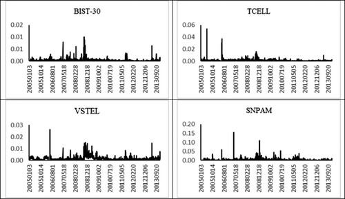
Figure 2. Intraday realised volatility. This table shows intraday realised volatility from 9.15 to 17.40 for BIST-30 and individual stocks in the non-crisis periods and the crisis period. Individual stocks are TCELL, VSTEL and SNPAM, which represent big, medium and small stocks respectively. The data sample ranges from January 1, 2005 to December 31, 2013, including 2,268 trading days. The intraday interval is five minutes. The crisis period considered in this paper is from July 19, 2007 to May 29, 2009.

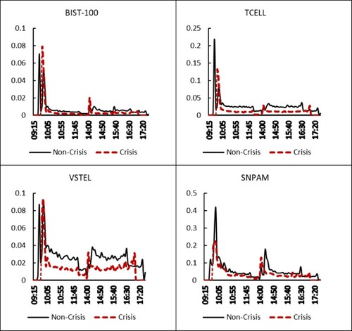
Figure 3. Intraday periodicity-adjusted jump statistics. This table shows summary statistics of the periodicity-adjusted intraday jump tests of Andersen, Bollerslev, and Diebold (2007b) for BIST-30 and individual stocks in the non-crisis periods and the crisis period. Individual stocks are TCELL, VSTEL and SNPAM, which represent big, medium and small stocks respectively. The data sample ranges from January 1, 2005 to December 31, 2013, including 2,268 trading days. The intraday interval is five minutes. The crisis period considered in this paper is from July 19, 2007 to May 29, 2009.

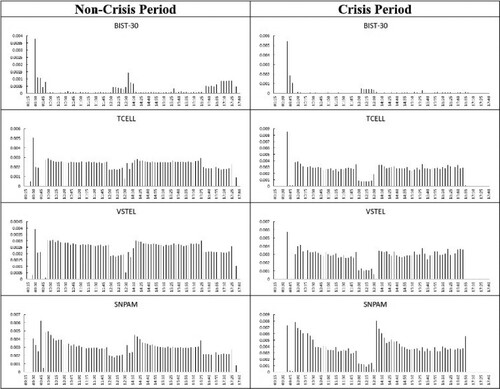
Figure 4. Sample distribution of S_W statistics. This figure shows the distribution of the non-standardised statistics for Brownian motion given by S_w for BIST-30 and TCELL, which represent the stock market index and big stocks respectively in the non-crisis periods and the crisis period. The table is obtained by computing the S_w, using values of k=2, α=2, and 1≤p≤1.75, taking into account asymmetry effects. The data sample ranges from January 1, 2005 to December 31, 2013, including 2,268 trading days. The intraday interval is five minutes. The crisis period considered in this paper is from July 19, 2007 to May 29, 2009.

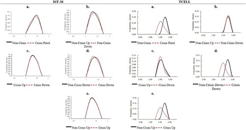
Figure 5. Sample distribution of S_W statistics. This figure shows the distribution of the non-standardised statistics for Brownian motion given by S_w for VSTEL and SNPAM, which represent medium and small stocks respectively in the non-crisis periods and the crisis period. The table is obtained by computing the S_w, using values of k=2, α=2, and 1≤p≤1.75, taking into account asymmetry effects. The data sample ranges from January 1, 2005 to December 31, 2013, including 2,268 trading days. The intraday interval is five minutes. The crisis period considered in this paper is from July 19, 2007 to May 29, 2009.

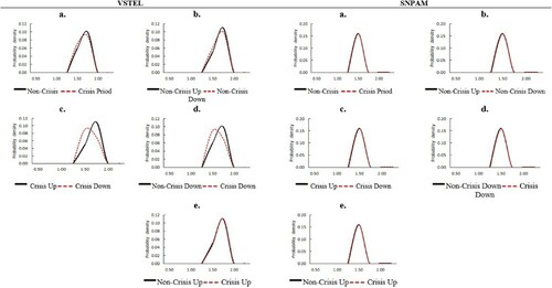
Figure 6. Intraday distribution of S_W statistics. This figure shows the intraday distribution of the non-standardised statistics for Brownian motion given by S_w for BIST-30 and TCELL, which represent the stock market index and big stock respectively in the non-crisis periods and the crisis period. The table is obtained by computing the S_w, using values of k=2, α=2, and 1≤p≤1.75, taking into account asymmetry effects. The data sample ranges from January 1, 2005 to December 31, 2013, including 2,268 trading days. The intraday interval is five minutes. The crisis period considered in this paper is from July 19, 2007 to May 29, 2009.

Figure 7. Intraday distribution of S_W statistics. This figure shows the intraday distribution of the non-standardised statistics for Brownian motion given by S_w for VSTEL and SNPAM, which represent medium and small stocks respectively in the non-crisis periods and the crisis period. The table is obtained by computing the S_w, using values of k=2, α=2, and 1≤p≤1.75, taking into account asymmetry effects. The data sample ranges from January 1, 2005 to December 31, 2013, including 2,268 trading days. The intraday interval is five minutes. The crisis period considered in this paper is from July 19, 2007 to May 29, 2009.

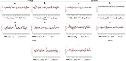
Figure 8. Sample distribution of S_j statistics. This figure shows the distribution of the non-standardised statistics for the presence of jumps given by S_j for BIST-30 and TCELL, which represent the stock market index and big stock in the non-crisis periods and the crisis period. The table is obtained by computing the S_j, using values of k=2, α=8, and 2≤p≤6, taking into account asymmetry effects. The data sample ranges from January 1, 2005 to December 31, 2013, including 2,268 trading days. The intraday interval is five minutes. The crisis period considered in this paper is from July 19, 2007 to May 29, 2009.

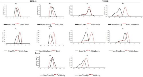
Figure 9. Sample distribution of S_j statistics. This figure shows the distribution of the non-standardised statistics for the presence of jumps given by S_j for VSTEL and SNPAM, which represent medium and small stocks respectively in the non-crisis periods and the crisis period. The table is obtained by computing the S_j, using values of k=2, α=8, and 2≤p≤6, taking into account asymmetry effects. The data sample ranges from January 1, 2005 to December 31, 2013, including 2,268 trading days. The intraday interval is five minutes. The crisis period considered in this paper is from July 19, 2007 to May 29, 2009.

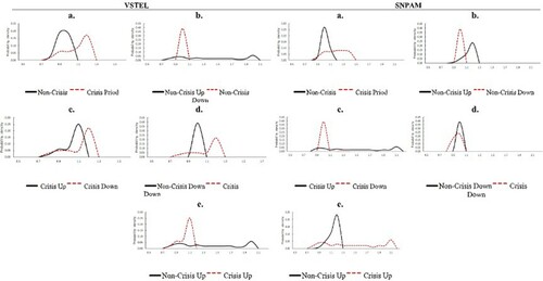
Figure 10. Intraday distribution of S_j statistics. This figure shows the intraday distribution of the non-standardised statistics for the presence of jumps given by S_j for BIST-30 and TCELL, which represent the stock market index and big stock in the non-crisis periods and the crisis period. The table is obtained by computing the S_j, using values of k=2, α=8, and 2≤p≤6, taking into account asymmetry effects. The data sample ranges from January 1, 2005 to December 31, 2013, including 2,268 trading days. The intraday interval is five minutes. The crisis period considered in this paper is from July 19, 2007 to May 29, 2009.

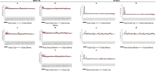
Figure 11. Intraday distribution of S_j statistics. This figure shows the intraday distribution of the non-standardised statistics for the presence of jumps given by S_j for VSTEL and SNPAM, which represent medium and small stocks respectively in the non-crisis periods and the crisis period. The table is obtained by computing the S_j, using values of k=2, α=8, and 2≤p≤6, taking into account asymmetry effects. The data sample ranges from January 1, 2005 to December 31, 2013, including 2,268 trading days. The intraday interval is five minutes. The crisis period considered in this paper is from July 19, 2007 to May 29, 2009.

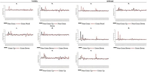
Figure 12. Sample distribution of S_FA statistics. This figure shows the distribution of the non-standardised statistics that distinguish between finite and infinite jumps given by S_FA for BIST-30 and TCELL, which represent big stocks in the non-crisis periods and the crisis period. The table is obtained by computing the S_FA, using values of k=2, α=8, and 2≤p≤6, taking into account asymmetry effects. The data sample ranges from January 1, 2005 to December 31, 2013, including 2,268 trading days. The intraday interval is five minutes. The crisis period considered in this paper is from July 19, 2007 to May 29, 2009.

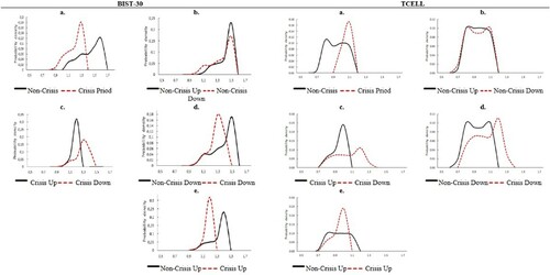
Figure 13. Sample distribution of S_FA statistics. This figure shows the distribution of the non-standardised statistics that distinguish between finite and infinite jumps given by S_FA for VSTEL and SNPAM, which represent medium and small stocks respectively in the non-crisis periods and the crisis period. The table is obtained by computing the S_FA, using values of k=2, α=8, and 2≤p≤6, taking into account asymmetry effects. The data sample ranges from January 1, 2005 to December 31, 2013, including 2,268 trading days. The intraday interval is five minutes. The crisis period considered in this paper is from July 19, 2007 to May 29, 2009.

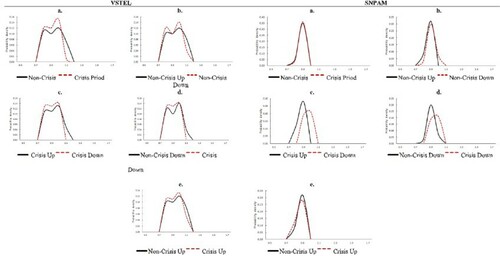
Figure 14. Intraday distribution of S_FA statistics. This figure shows the intraday distribution of the non-standardised statistics that distinguish between finite and infinite jumps given by S_FA for BIST-30 and TCELL, which represent the stock market index and big stocks in the non-crisis periods and the crisis period. The table is obtained by computing the S_FA, using values of k=2, α=8, and 2≤p≤6, taking into account asymmetry effects. The data sample ranges from January 1, 2005 to December 31, 2013, including 2,268 trading days. The intraday interval is five minutes. The crisis period considered in this paper is from July 19, 2007 to May 29, 2009.

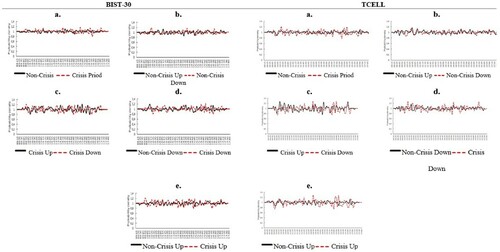
Figure 15. Intraday distribution of S_FA statistics. This figure shows the intraday distribution of the non-standardised statistics that distinguish between finite and infinite jumps given by S_FA for VSTEL and SNPAM, which represent medium and small stocks respectively in the non-crisis periods and the crisis period. The table is obtained by computing the S_FA, using values of k=2, α=8, and 2≤p≤6, taking into account asymmetry effects. The data sample ranges from January 1, 2005 to December 31, 2013, including 2,268 trading days. The intraday interval is five minutes. The crisis period considered in this paper is from July 19, 2007 to May 29, 2009.

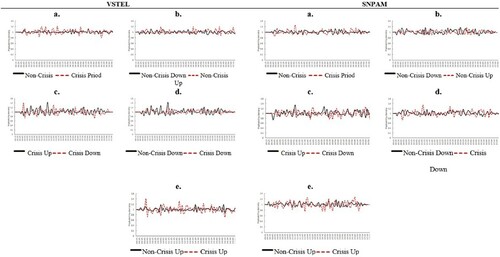
Figure 16. Activity signature plots. This figure shows quantile activity signature functions computed for BIST-30 and TCELL, which represent the stock market index and big stock respectively in the non-crisis periods and the crisis period. The table is obtained by computing the function using values of p for the quantiles using 0.25 (for lower bound), 0.50 (for median), and 0.75 for upper bound, taking into account asymmetry effects. The data sample ranges from January 1, 2005 to December 31, 2013, including 2,268 trading days. The intraday interval is five minutes. The crisis period considered in this paper is from July 19, 2007 to May 29, 2009.

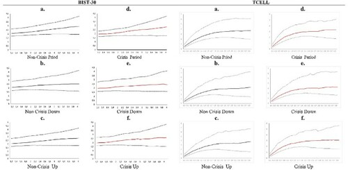
Figure 17. Activity signature plots. This figure shows quantile activity signature functions computed for VSTEL and SNPAM, which represent medium and small stocks respectively in the non-crisis periods and the crisis period. The table is obtained by computing the function using values of p for the quantiles using 0.25 (for lower bound), 0.50 (for median), and 0.75 for upper bound, taking into account asymmetry effects. The data sample ranges from January 1, 2005 to December 31, 2013, including 2,268 trading days. The intraday interval is five minutes. The crisis period considered in this paper is from July 19, 2007 to May 29, 2009.

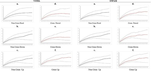
Table 5. The proportion of quadratic variation.

	Non-crisis period			Crisis period
	Continuous	Jump		Continuous	Jump
	BIST-30
		Big J.	Small J.		Big J.	Small J.
Non Asymmetry	0.79	0.09	0.12	0.64	0.22	0.14
Up Asymmetry	0.82	0.07	0.11	0.71	0.19	0.10
Down Asymmetry	0.47	0.47	0.08	0.60	0.23	0.17
	TCELL
Non Asymmetry	0.88	0.04	0.08	0.83	0.08	0.09
Up Asymmetry	0.93	0.02	0.05	0.84	0.09	0.07
Down Asymmetry	0.83	0.13	0.04	0.82	0.09	0.09
	VSTEL
Non Asymmetry	0.92	0.05	0.03	0.88	0.08	0.04
Up Asymmetry	0.92	0.02	0.06	0.86	0.05	0.09
Down Asymmetry	0.57	0.41	0.02	0.90	0.04	0.06
	SNPAM
Non Asymmetry	0.70	0.16	0.14	0.74	0.20	0.6
Up Asymmetry	0.71	0.10	0.19	0.75	0.03	0.22
Down Asymmetry	0.53	0.38	0.09	0.73	0.10	0.17

Note: This table shows what fraction of the quadratic variation is attributable to the continuous and jump components for BIST-30 and individual stocks in the non-crisis periods and the crisis period. Individual stocks are TCELL, VSTEL and SNPAM, which represent big, medium and small stocks respectively. This table is obtained by computing the fraction of quadratic variation from the Brownian component, using values of ω=1/2, α=8 and ε=2α. The data sample ranges from January 1, 2005 to December 31, 2013, including 2,268 trading days. The intraday interval is five minutes. The crisis period considered in this paper is from July 19, 2007 to May 29, 2009.

Figure 18. The distribution of S_TI, S^Minus_TI, and S^Plus_TI statistics. This figure shows the distribution of the non-standardised statistics for the presence of large jumps given by S_TI, S^Minus_TI, and S^Plus_TI for TCELL, VSTEL and SNPAM, which represent big, medium and small stocks respectively in the non-crisis periods and the crisis period. The table is obtained by computing the statistics of S_TI, S^Minus_TI, and S^Plus_TI, using values of 2.1≤p≤6, α=2, and k=2. The data sample ranges from January 1, 2005 to December 31, 2013, including 2,268 trading days. The intraday interval is five minutes. The crisis period considered in this paper is from July 19, 2007 to May 29, 2009.

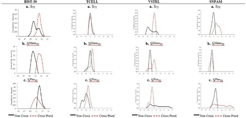
Table 6. The Kolmogorov-Smirnov (KS) test.

	BIST-30	TCELL	VSTEL	SNPAM
Non-Crisis Period-Crisis Period
SJ	3.242 (0.000)	1.789 (0.003)	3.130 (0.000)	3.354 (0.000)
SFA	2.460 (0.000)	0.894 (0.400)	0.671 (0.759)	0.335 (0.998)
SW	0.354 (0.998)	1.945 (0.001)	0.354 (0.998)	1.061 (0.211)
STI	3.130 (0.000)	1.118 (0.164)	3.446 (0.000)	4.472 (0.000)
STI^Minus	4.472 (0.000)	2.907 (0.000)	3.242 (0.000)	4.025 (0.000)
STI^Plus	2.907 (0.000)	3.130 (0.000)	3.355 (0.000)	3.354 (0.000)
Non-Crisis Up-Crisis Down
SJ	4.249 (0.000)	4.025 (0.000)	2.907 (0.000)	3.919 (0.000)
SFA	2.236 (0.000)	1.901 (0.001)	1.230 (0.097)	3.130 (0.000)
SW	0.177 (0.998)	2.121 (0.000)	0.884 (0.415)	2.475 (0.000)
Crisis Up-Crisis Down
SJ	3.354 (0.000)	3.578 (0.000)	2.571 (0.000)	4.137 (0.000)
SFA	3.578 (0.000)	2.571 (0.000)	1.006 (0.263)	3.578 (0.000)
SW	0.354 (0.000)	0.530 (0.941)	0.707 (0.699)	2.474 (0.000)
Non Crisis Down-Crisis Down
SJ	4.471 (0.000)	2.683 (0.000)	3.019 (0.000)	3.801 (0.000)
SFA	2.795 (0.000)	1.789 (0.003)	0.894 (0.400)	2.124 (0.000)
SW	0.177 (0.998)	2.298 (0.000)	0.530 (0.941)	1.591 (0.013)
Non Crisis Up-Crisis Up
SJ	2.683 (0.000)	3.019 (0.000)	3.120 (0.000)	3.354 (0.000)
SFA	3.690 (0.000)	1.342 (0.055)	0.335 (0.998)	1.677 (0.007)
SW	0.176 (0.998)	1.591 (0.013)	0.177 (0.998)	0.354 (0.998)

Note: This table shows the KS results for BIST-30 and individual stocks, taking into account the asymmetry effects. Individual stocks are TCELL, VSTEL and SNPAM, which represent big, medium and small stocks respectively. KS tests whether the distribution of statistics such as S_J S_FA S_W S_TI S_TI^Minus S_TI^Plus for the data-generating process is statistically the same for the related sub-period. If F₁(x) and F₂(x) are the respective cumulative density functions, H0= F₁(x) = F₂(x) H1= F₁(x) ≠ F₂(x). The data sample ranges from January 1, 2005 to December 31, 2013, including 2,268 trading days. The crisis period considered in this paper is from July 19, 2007 to May 29, 2009.

Figure 19. This figure shows the intraday distribution of the non-standardised statistics for the presence of large jumps given by S_TI, S^Minus_TI, and S^Plus_TI for TCELL, VSTEL and SNPAM, which represent big, medium and small stocks respectively in the non-crisis periods and the crisis period. The table is obtained by computing the statistics of S_TI, S^Minus_TI, and S^Plus_TI, using values of 2.1≤p≤6, α=2, and k=2. The data sample ranges from January 1, 2005 to December 31, 2013, including 2,268 trading days. The intraday interval is five minutes. The crisis period considered in this paper is from July 19, 2007 to May 29, 2009.

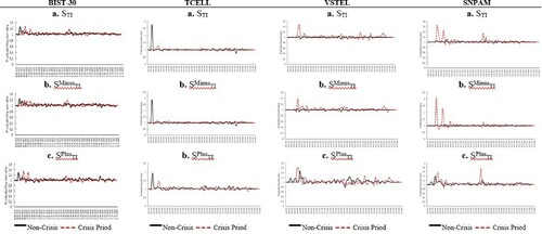
Table 7. Stressful days for absolute tail.

2005	2006	2007	2008	2009	2010	2011	2012	2013
BIST-30
16-Feb	12-May		23-Jan			9-Aug		23-May
06-Oct	16-May		28-Jan					4-Jun
	8-Jun		8-Sep					25-Jun
	20-July		15-Sep					22-Aug
	25-July		26-Sep					25-Dec
			6-Oct					31-Dec
			13-Oct
			24-Nov
				TCELL
28-Jan	20-Jan		21-Jan	-		24-Feb		25-Jan
19-Apr	14-Jun		13-Feb			30-Sep
	13-July
				VSTEL
			17-Mar	12-Oct		10-Jan	20-Jan	28-Jun
			6-Oct			18-Apr	14-May	18-Jul
			13-Oct			8-Aug		30-Oct
						11-Aug		31-Dec
				SNPAM
	11-Dec	14-Jun	17-Mar	21-Jan	23-Jun	11-Jul	10-Feb	06-Sep
		15-Oct	21-Oct	29-Jun		27-Sep
			16-Dec

Note: The table reports the stressful days for absolute tail, identified as stressful with the I_stress (p, u_n, k, Δ _n) in the paper, using four standard deviations over the median as the threshold value. Stressful days are detected for BIST-30 and individual stocks. Individual stocks are TCELL, VSTEL and SNPAM, which represent big, medium and small stocks respectively. The data sample ranges from January 1, 2005 to December 31, 2013, including 2,268 trading days. The intraday interval is five minutes. The crisis period considered in this paper is from July 19, 2007 to May 29, 2009.

Table 8. Stressful days for positive tail.

2005	2006	2007	2008	2009	2010	2011	2012	2013
BIST-30
12-Apr	16-May	30 Apr	24-Jan					4-Jun
20-Oct			8-Sep					25-Jun
			17-Sep					2-Sep
			8-Oct
			24-Nov
				TCELL
28-Jan	20-Jan		23-Jan
19-Apr	15-Mar		27-Feb
	13-Jun		28-Feb
	14-Jun		30 Jul
	05-Oct		23-Oct
	07-Dec
				VSTEL
			13-Oct	05-Jun		11-Aug	10-Jan	18-Jul
							20-Jan	30-Oct
							14-May
				SNPAM
			21-Oct	24-Feb	23-Jun	27-Sep	10-Feb	11-Apr
								06-Sep

Note: The table reports the stressful days for positive tail identified as stressful with the I_stress (p, u_n, k, Δ _n) in the paper, using four standard deviations over the median as the threshold value. Stressful days are detected for BIST-30 and individual stocks. Individual stocks are TCELL, VSTEL and SNPAM, which represent big, medium and small stocks respectively. The data sample ranges from January 1, 2005 to December 31, 2013, including 2,268 trading days. The intraday interval is five minutes. The crisis period considered in this paper is from July 19, 2007 to May 29, 2009.

Table 9. Stressful days for negative tail.

2005	2006	2007	2008	2009	2010	2011	2012	2013
BIST-30
17-Mar	8-Jun		15-Sep			9-Aug		6-Jun
								22-Aug
								25-Dec
				TCELL
02-Feb	08-Mar		28-Jan			24-Feb
23-May	06-Jul		08-May			30-Sep
			03-Oct
			16-Oct
				VSTEL
			23-Jan			18-Apr		25-Dec
			14-Mar			08-Aug		31-Dec
			06-Oct
				SNPAM
	24-Mar	14-Jun	17-Mar	24-Feb	06-Jan	11-Aug
	11-Aug		16-Oct	17-Oct	23-Jun	27-Sep

Note: The table reports the stressful days for negative tail, identified as stressful with the I_stress (p, u_n, k, Δ _n) in the paper, using four standard deviations over the median as the threshold value. Stressful days are detected for BIST-30 and individual stocks. Individual stocks are TCELL, VSTEL and SNPAM, which represent big, medium and small stocks respectively. The data sample ranges from January 1, 2005 to December 31, 2013, including 2,268 trading days. The intraday interval is five minutes. The crisis period considered in this paper is from July 19, 2007 to May 29, 2009.

Andersen, T. G., T. Bollerslev, and F. X. Diebold. 2007b. “Roughing it up: Including Jump Components in the Measurement, Modeling, and Forecasting of Return Volatility.” The Review of Economics and Statistics 89 (4): 701–720.

 Web of Science ®Google Scholar

Data availability statement

The data that support the findings of this study are available from the corresponding author upon reasonable request.