Figures & data
Table 1. Descriptive statistics.
Table 2. Connectedness – Full sample.
Figure 1. Dynamic total spillover index.
Notes: This Figure displays the time-varying behaviour of the total connectedness index between international monetary policy and cryptocurrency returns. It is based on the generalised forecast-error variance decomposition (GFEVD) obtained from the estimation of a TVP-VAR model of order 2 and 10-step ahead forecasts. The sample period is August 5, 2013 – September 27, 2019. The lag length is selected in accordance with the (minimum value of the) Bayesian information criterion (BIC).
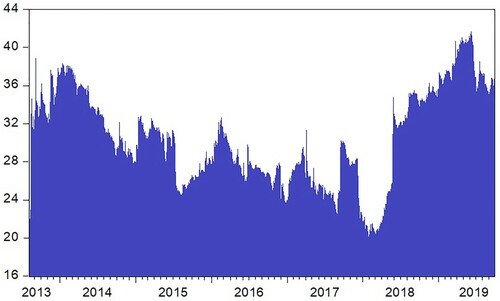
Figure 2. Dynamic gross directional spillovers TO others.
Notes: This Figure displays the time-varying behaviour of the gross directional spillovers from each underlying variable TO all other variables. It is based on the generalised forecast-error variance decomposition (GFEVD) obtained from the estimation of a TVP-VAR model of order 2 and 10-step ahead forecasts. The sample period is August 5, 2013 – September 27, 2019. The lag length is selected in accordance with the Bayesian information criterion (BIC).
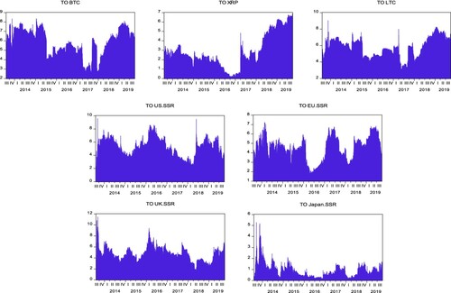
Figure 3. Dynamic gross directional spillovers FROM others.
Notes: This Figure displays the time-varying behaviour of the gross directional spillovers to each underlying variable FROM all other variables. It is based on the generalised forecast-error variance decomposition (GFEVD) obtained from the estimation of a TVP-VAR model of order 2 and 10-step ahead forecasts. The sample period is August 5, 2013 – September 27, 2019. The lag length is selected in accordance with the Bayesian information criterion (BIC).
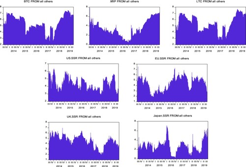
Figure 4. Dynamic net directional spillover indices.
Notes: This Figure displays the time-varying behaviour of the net directional spillovers from each underlying variable to all other variables. Positive (negative) values indicate that the variable under consideration is a net transmitter (receiver) of spillovers to (from) all other variables. Spillovers are based on the generalised forecast-error variance decomposition (GFEVD) obtained from the estimation of a TVP-VAR model of order 2 and 10-step ahead forecasts. The sample period is August 5, 2013 – September 27, 2019. The lag length is selected in accordance with the Bayesian information criterion (BIC).
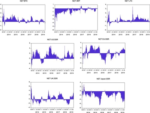
Figure 5. Network of directional pairwise spillovers.
Notes: This Figure portrays the net directional pairwise spillovers among all possible pairs of variables. A node’s colour identifies if a variable is a net transmitter/receiver of shocks to/from other variables. The red (green) colour indicates that the variable is a net transmitter (receiver) of spillovers. Furthermore, the thickness and the colour of the arrows represent the magnitude and strength of the average spillover between each pair, respectively. In this case, the navy colour of the arrows indicates strong spillovers, the blue colour shows moderate spillovers, and the light blue colour refers to weak spillovers. Spillovers are based on the generalised forecast-error variance decomposition (GFEVD) obtained from the estimation of a TVP-VAR model of order 2 and 10-step ahead forecasts. The sample period is August 5, 2013 – September 27, 2019. The lag length is selected in accordance with the Bayesian information criterion (BIC).
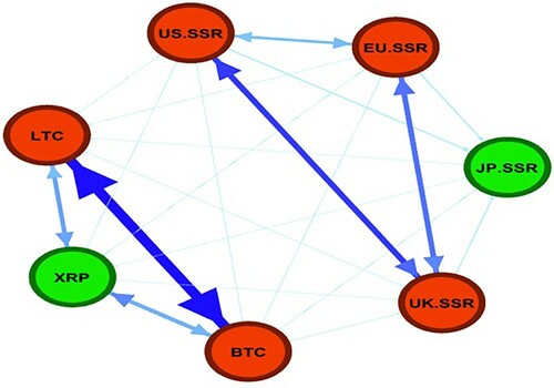
Table 3. Connectedness – Unconventional monetary policy (August 5, 2013 – December 16, 2015).
Table 4. Connectedness – Conventional monetary policy (December 17, 2015 – September 27, 2019).
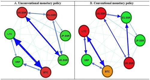
Figure 6. Network of directional pairwise spillovers – Conventional versus unconventional monetary policy.
Notes: Panels A and B portray the net directional pairwise spillovers among all possible pairs of variables. A node’s colour identifies if a variable is a net transmitter/receiver of shocks to/from other variables. The red (green) colour indicates that the variable is a net transmitter (receiver) of spillovers, while the light brown colour indicates that the variable is neutral. Furthermore, the thickness and the colour of the arrows represent the magnitude and strength of the average spillover between each pair, respectively. In this case, the navy colour of the arrows indicates strong spillovers, the blue colour shows moderate spillovers, and the light blue colour refers to weak spillovers. Spillovers are based on the generalised forecast-error variance decomposition (GFEVD) obtained from the estimation of a TVP-VAR model of order 2 and 10-step ahead forecasts. The sub-sample periods are August 5, 2013 – December 16, 2015 and December 17, 2015 – September 27, 2019. The lag length is selected in accordance with the Bayesian information criterion (BIC).