Portfolio optimization beyond utility maximization: the case of driftless markets

Figures & data

Figure 1. Log returns of the exchange rates of selected currencies in terms of EUR, where the black region is 95% confidence interval and the red region is the 50% confidence interval as implied by the market volatility. Note that the log returns of most currencies stay in the tighter 50% confidence interval, indicating slight mean reversion. Several currencies exhibit a drift: CZK, HUF, CHF, and ZAR.

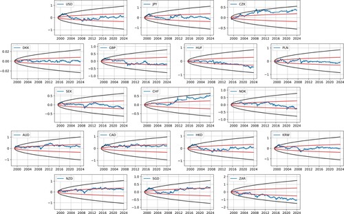
Figure 2. Distributional opinions about the final value of the log return $\log \left(\frac{X_Y\left(T\right)}{X_Y\left(0\right)}\right)$ from the perspective of the two currencies ${\mathbb{P}}^X$ and ${\mathbb{P}}^Y$, their index ${\mathbb{P}}^I$, and the subjective agent's opinion ${\mathbb{P}}^M$ with parameters ${\sigma }_q=0.1$, ${\sigma }_p=0.08$, and T = 25.

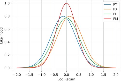
Figure 3. Likelihood ratios corresponding to the final log return $\log \left(\frac{X_Y\left(T\right)}{X_Y\left(0\right)}\right)$ of the subjective agent's opinion ${\mathbb{P}}^M$ against three available benchmarks: ${\mathbb{P}}^Y$, ${\mathbb{P}}^X$, and ${\mathbb{P}}^I$ from Figure 2 together with the rejection regions based on the Neyman-Pearson lemma. The central regions reject the state price density of the reference currency, the tail regions reject the state price density of the agent.

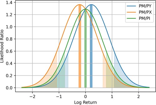
Table 1. Final log return $\log \left(\frac{X_Y\left(T\right)}{X_Y\left(0\right)}\right)$ as the test statistics of the exchange rate together with the rejection regions corresponding to all 3 different benchmarks. FX rates of currencies in bold stayed statistically significant around zero.

	LogR	Index	EUR	FX
USD	0.06	−[0.03, 0.03]	[0.16, 0.24]	[−0.24, −0.16]
JPY	−0.16	[−0.04, 0.04]	[0.25, 0.35]	[−0.35, −0.25]
CZK	0.35	[−0.02, 0.02]	[0.05, 0.09]	[−0.09, −0.05]
DKK	−0.00	[−0.00,0.00]	[−0.00, 0.00]	[−0.00,0.00]
GBP	−0.20	[−0.03, 0.03]	[0.11, 0.17]	[−0.17, −0.11]
HUF	−0.42	[−0.03,0.03]	[0.13, 0.20]	[−0.20, −0.13]
PLN	−0.06	[−0.03, 0.03]	[0.14, 0.21]	[−0.21, −0.14]
SEK	−0.16	[−0.02, 0.02]	[0.07, 0.12]	[−0.12, −0.07]
CHF	0.56	[−0.02, 0.02]	[0.07, 0.12]	[−0.12, −0.07]
NOK	−0.24	[−0.03, 0.03]	[0.11, 0.17]	[−0.17, −0.11]
AUD	0.16	[−0.03, 0.03]	[0.20, 0.28]	[−0.28, −0.20]
CAD	0.21	[−0.03, 0.03]	[0.17, 0.25]	[−0.25, −0.17]
HKD	0.06	[−0.03, 0.03]	[0.16,0.24]	[−0.24, −0.16]
KRW	−0.02	[−0.04, 0.04]	[0.23, 0.33]	[−0.33, −0.23]
NZD	0.24	[−0.04, 0.04]	[0.22, 0.31]	[−0.31, −0.22]
SGD	0.29	[−0.02, 0.02]	[0.10, 0.16]	[−0.16, −0.10]
ZAR	−1.08	[−0.05, 0.05]	[0.44, 0.60]	[−0.60, −0.44]

Table 2. Optimal values of the portfolios as a result of log utility maximization denominated in the index of two currencies, EUR, and the foreign currency.

	Index	EUR	FX
USD	1.280	1.321	1.239
JPY	1.281	1.181	1.380
CZK	0.826	0.970	0.683
DKK	1.250	1.249	1.250
GBP	1.192	1.073	1.312
HUF	0.998	0.791	1.204
PLN	1.274	1.233	1.315
SEK	1.188	1.094	1.282
CHF	0.595	0.756	0.433
NOK	1.161	1.023	1.299
AUD	1.263	1.364	1.161
CAD	1.230	1.356	1.103
HKD	1.281	1.317	1.245
KRW	1.299	1.283	1.316
NZD	1.237	1.384	1.089
SGD	1.089	1.247	0.930
ZAR	0.885	0.450	1.320

Note: Bold values indicate statistical significance. All statistically significant payoffs favor the hypothesis of smaller volatility with the exceptions of the CHF portfolio denominated in CHF and the Index and the ZAR portfolio denominated in EUR.

Figure 4. The time evolution of the optimal value function for all currencies benchmarked with respect to EUR (blue graph), the other currency (orange graph), and the index of the two currencies (green graph). The choice of the scaling factor a in ${\sigma }_p=a\cdot {\sigma }_q$ is 0.8.

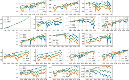
Figure 5. Comparison of the EUR theoretical optimal value function (blue) with its replicating portfolio (red).

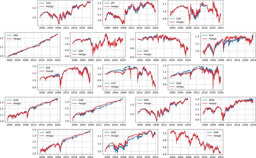
Table 3. Annualized Sharpe ratio.

	Index	EUR	FX
USD	0.454	0.241	0.180
JPY	0.542	0.159	0.214
CZK	−0.048	0.013	−0.078
DKK	0.906	0.906	0.894
GBP	0.214	0.075	0.337
HUF	0.023	−0.060	0.209
PLN	0.684	0.200	0.259
SEK	0.279	0.098	0.304
CHF	−0.198	−0.135	−0.221
NOK	0.200	0.046	0.268
AUD	0.314	0.422	0.113
CAD	0.250	0.710	0.089
HKD	0.456	0.237	0.185
KRW	0.551	0.196	0.208
NZD	0.276	0.419	0.083
SGD	0.108	0.318	−0.002
ZAR	−0.064	−0.149	0.264

Figure 6. The performance of individual funds as a function of the scaling parameter a for different currencies denominated in EUR. Currencies with smaller variability peak for values under a = 1. The red line corresponds to the mean performance of the funds sampled from the $\mathrm{\Gamma }(4,8)$ distribution for the scaling factor a.

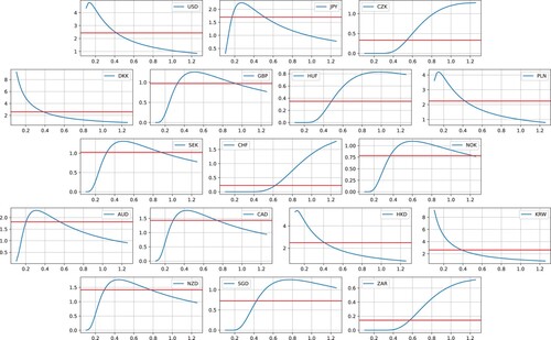
Table 4. Cumulative performance of the Bayesian portfolios.

	Index	EUR	FX
USD	2.360	2.436	2.284
JPY	1.840	1.697	1.984
CZK	0.285	0.335	0.236
DKK	2.585	2.585	2.586
GBP	1.079	0.971	1.187
HUF	0.440	0.349	0.531
PLN	2.314	2.240	2.388
SEK	1.114	1.026	1.202
CHF	0.178	0.227	0.130
NOK	0.890	0.784	0.996
AUD	1.677	1.812	1.543
CAD	1.296	1.429	1.162
HKD	2.422	2.490	2.354
KRW	2.669	2.636	2.702
NZD	1.266	1.417	1.116
SGD	0.632	0.724	0.541
ZAR	0.280	0.142	0.417

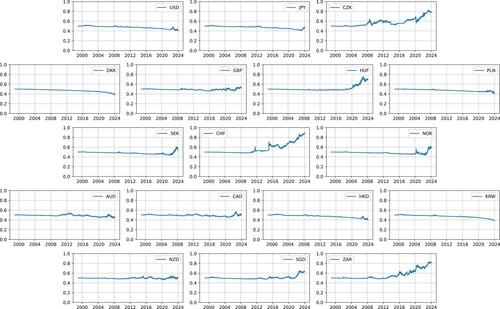
Figure 7. Temporal evolution of the mean posterior for the scaling factor parameter a.

Data Availability Statement

The data that support the findings of this study are openly available in the European Central Bank repository at https://www.ecb.europa.eu/stats/eurofxref/eurofxref-hist.zip, derived from the European Central Bank Exchange Rate Data.