Rental Market Liquidity, Seasonality, and Distance to Universities

Figures & data

Table 1. Sample characteristics.

	Rental Price		Distance to the closest campus*		TOM (in months)*		Number of bedrooms
	Mean	Std. Dev.	Mean	Std. Dev.	Mean	Std. Dev.	Mean	Std. Dev.
Birmingham	167.72	79.00	4.59	4.16	2.05	1.76	2.27	1.33
Bristol	224.23	95.35	3.92	3.74	1.81	1.19	2.13	1.23
Cardiff	190.23	110.14	4.59	5.58	2.13	1.77	2.65	1.76
Coventry	195.02	100.18	5.80	5.61	2.15	1.70	2.33	1.24
Edinburgh	219.71	105.77	4.18	4.83	1.48	0.91	2.11	1.01
Glasgow	160.44	74.58	4.38	4.43	1.67	0.95	1.93	0.84
Leeds	195.11	123.07	3.33	3.34	2.34	2.12	2.69	1.77
Liverpool	152.38	87.03	3.90	3.26	2.32	2.15	2.33	1.27
Manchester	191.24	102.14	4.01	2.93	1.94	1.41	2.36	1.34
Newcastle	164.50	100.65	5.43	5.03	2.31	2.18	2.57	1.29
Nottingham	162.93	99.69	5.49	5.99	2.06	1.52	2.50	1.35
Plymouth	159.52	73.91	3.65	4.17	2.16	1.51	2.18	1.19
Sheffield	141.72	71.39	8.17	6.98	2.18	1.69	2.23	1.17
Sample	178.36	98.74	4.74	4.82	2.06	1.72	2.36	1.34
3-km range	200.02	114.71	1.55	0.79	2.19	2.00	2.41	1.58

Note: This table presents the descriptive statistics of the sample. Rental price refers to weekly rent. We ignore the change in price and calculate mean value from the price from first time the listing is published. *As the crow flies-point to point straight line- distance between a listing and nearest university campus in term of kilometres, **length of time that a listing stays on market.

Figure 1. Ratio of exit to available by months.

Note: Figure reports the exit ratio, calculated by dividing the number of listings exiting the market in a calendar month by the total number of existing listings in relevant calendar month regardless of year. Time span is the period from August 2015 to August 2017 period. Each Grey shaded line represents one of 13 cities included in the sample. The dark solid line represents the ratio for the whole sample. Figures for individual cities are presented in Online Appendix.

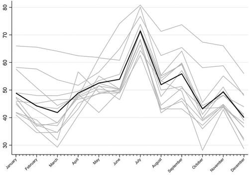
Figure 2. Average time on market (in months).

Note: Figure 2 represents time on market. Each point on the line provides the average length of marketing time of the listings that come to the market in relevant month. The dashed-black line represents the listings which are within 3-km distance to a university campus. The solid grey line represents the listings which are more than 3-km away from a university campus.

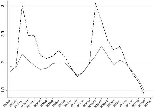
Figure 3. Price change over time.

Note: Figure 2 represents the coefficients from two-period rolling-time-dummy OLS regressions. The dependent variable in the regression is log-weekly rental price. Each regression includes 2 sequential months only to capture changes in prices after controlling for size and city. For instance, in the first regression, listings that come to market in August 2015 and September 2015 are included where a dummy for September 2015 listings is added as a regressor. Second regression excludes August 2015 listings, includes October 2015 listings and accordingly a dummy for October 2015 listings is included in the regression. Same procedure is repeated for each month of the sample period. All regressions include variables to control for number of bedrooms and city of listing. Thin black line represents the listings which are more than 3-km away from a university campus. Thick blue line represents listings which are within 3-km distance to a university campus.

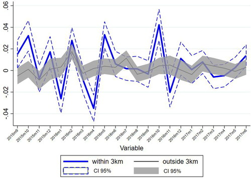
Table 2. Regression results- 3-km sample vs full sample (Dependent Variable: Dummy variable indicating the exit from market).

	Cloglog		Panel Cloglog
Variables	3-km	Full	3-km	Full
N. of bedrooms	−0.040***	−0.039***	−0.038***	−0.037***
	(0.002)	(0.002)	(0.002)	(0.002)
Weekly rent (log)	−0.038***	−0.041***	−0.026***	−0.032***
	(0.004)	(0.003)	(0.005)	(0.003)
N. of rental ads in outcode (log)	−0.075***	−0.071***	−0.106***	−0.098***
	(0.003)	(0.003)	(0.004)	(0.003)
N. of sale ads in outcode (log)	0.036***	0.050***	0.051***	0.065***
	(0.005)	(0.003)	(0.005)	(0.004)
Distance to closest campus (log)	0.057***	−0.007***	0.049***	−0.024***
	(0.005)	(0.003)	(0.005)	(0.003)
February	−0.171***	−0.168***	−0.170***	−0.170***
	(0.012)	(0.009)	(0.012)	(0.009)
March	−0.263***	−0.244***	−0.264***	−0.247***
	(0.012)	(0.009)	(0.012)	(0.009)
April	0.122***	0.015*	0.127***	0.017**
	(0.011)	(0.008)	(0.012)	(0.008)
May	0.142***	0.070***	0.142***	0.070***
	(0.012)	(0.008)	(0.012)	(0.009)
June	0.210***	0.116***	0.206***	0.113***
	(0.012)	(0.009)	(0.012)	(0.009)
July	0.779***	0.651***	0.766***	0.641***
	(0.012)	(0.009)	(0.013)	(0.009)
August	0.231***	0.096***	0.218***	0.088***
	(0.015)	(0.010)	(0.015)	(0.011)
September	0.312***	0.166***	0.302***	0.163***
	(0.014)	(0.010)	(0.014)	(0.010)
October	−0.245***	−0.192***	−0.232***	−0.183***
	(0.014)	(0.010)	(0.014)	(0.010)
November	0.032**	−0.029***	0.056***	−0.012
	(0.013)	(0.010)	(0.013)	(0.010)
December	−0.314***	−0.358***	−0.305***	−0.352***
	(0.014)	(0.010)	(0.014)	(0.010)
2016	−0.143***	−0.134***	−0.139***	−0.131***
	(0.009)	(0.007)	(0.009)	(0.007)
2017	0.007	−0.011	0.016	−0.005
	(0.011)	(0.008)	(0.011)	(0.008)
Observations	342,968	618,913	157,508	300,198

Note: The first two columns provide the results from cross-sectional setting while last two columns provide panel data setting. The first and third columns present the result from sample that includes houses within 3-km distance from a university campus. The second and forth columns present full sample results. N. of rental ads in outcode (log) and N. of sale ads in outcode (log) variables capture the log of the number of rental and sale listings in the same outcode respectively. 11 dummy variables are included in the model for each calendar month except for January which serves as the base category. The coefficients for hazard function dummies, property type and cities are not reported for the sake of brevity. Results are available on request. *** p < 0.01, ** p < 0.05, * p < 0.1

Table 3. Regression results, interaction effects (Dependent Variable: Dummy variable indicating the exit from market).

	Cloglog		Panel Cloglog
Variables	Direct	Interaction	Direct	Interaction
Distance to closest campus (log)	0.046***		0.037***
	(0.006)		(0.006)
February	−0.195***	0.024***	−0.188***	0.016*
	(0.013)	(0.009)	(0.012)	(0.008)
March	−0.285***	0.038***	−0.281***	0.031***
	(0.013)	(0.009)	(0.013)	(0.009)
April	0.105***	−0.085***	0.116***	−0.093***
	(0.012)	(0.008)	(0.012)	(0.008)
May	0.142***	−0.067***	0.149***	−0.074***
	(0.012)	(0.008)	(0.012)	(0.008)
June	0.207***	−0.085***	0.210***	−0.090***
	(0.012)	(0.008)	(0.012)	(0.008)
July	0.762***	−0.103***	0.757***	−0.108***
	(0.013)	(0.009)	(0.013)	(0.009)
August	0.283***	−0.167***	0.277***	−0.170***
	(0.015)	(0.010)	(0.015)	(0.010)
September	0.390***	−0.188***	0.385***	−0.189***
	(0.014)	(0.009)	(0.014)	(0.009)
October	−0.238***	0.031***	−0.220***	0.023**
	(0.015)	(0.009)	(0.014)	(0.009)
November	0.019	−0.048***	0.048***	−0.061***
	(0.013)	(0.008)	(0.013)	(0.008)
December	−0.360***	−0.001	−0.344***	−0.011
	(0.014)	(0.009)	(0.014)	(0.009)
Observations	618,913		300,198

Note: The first two columns in the table present results from the cross-sectional setting while last two provides results from panel data setting. Interactions present the coefficients of the interaction terms between calendar months and minimum distance variable. Direct effect refers to the calendar month coefficients obtained after controlling for interactions. Same set of control variables as in Table 2 are included to interaction model. Full results are available on request. *** p < 0.01, ** p < 0.05, * p < 0.1.

Data statement

Our data were collected using Zoopla API service. Unfortunately, we cannot make our dataset public as the terms of use of the API (as of 2018) will be violated. Current terms (as of 2021) do not allow storing the data (https://developer.zoopla.co.uk/API_terms_of_use). A researcher who would like to replicate our study might consider applying for an alternative source of Zoopla data (e.g. through Urban Big Data Centre https://www.ubdc.ac.uk/). However, all Stata and Python codes available upon request from authors.