In situ strain investigation during laser welding using digital image correlation and finite-element-based numerical simulation

Figures & data

Figure 1. (a) Schematic of the laser bead-on-plate welding and DIC measurement set-up, (b) Typical emission spectra of an Nd:YAG laser plume on an iron-based specimen. The graph is replotted from [11]. The position of the optical narrow bandpass filter in this spectrum is also indicated, (c) Simulated and experimental temperature cycle. Here, T(1) refers to the measured temperature cycle at a distance of 3 mm from the weld centreline towards the free edge. T(2) and T(3) are the measured temperature cycles at a distance of 2.5 and 4 mm from the weld centreline towards the constrained edge.

Figure 2. Schematic of the 3D Gaussian conical heat source used in this work.

Figure 3. (a) Spatial distribution of transverse strain (in %) at t=3.0 s. Top image shows the distribution calculated using the FE-based model. The bottom image overlaying the speckle pattern shows the strain distribution measured using the DIC technique. The coordinate system used is the same as that used in Figure 1(a), (b) experimentally measured and numerically computed spatial distribution of transverse strain (in %) along the line H1 and H2 at t=1.75 s, (c) experimentally measured and numerically computed spatial distribution of transverse strain (in %) along the line H1 and H2 at t= 2.25 s, (d) experimentally measured and numerically computed temporal distribution of transverse strain (in %) at P1, (e) experimentally measured and numerically computed temporal distribution of transverse strain (in %) at P2, (f) experimentally measured and numerically computed temporal distribution of transverse strain (in %) at P3.

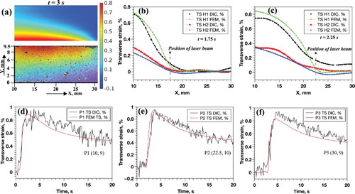
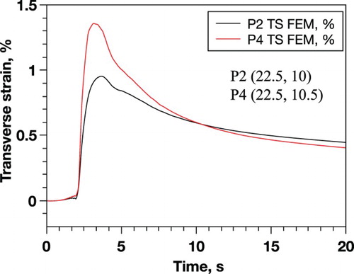
Figure 4. FEM-computed temporal distribution of transverse strain (in %) at P2 and P4.

Aalderink B, Aarts R, Jonker J, et al. Weld plume emissions during nd:yag laser welding. In: Beyer E, Dausinger F, Ostendorf A, et al., editors. Lasers in manufacturing 2005. München” AT-Fachverlag GmbH Stuttgart; 2005. p. 413–417.

 Google Scholar