Operators believe patient-specific rehearsal improve individual and team performance

Figures & data

Figure 1. The patient-specific rehearsal set-up with the VIST-LAB, VIST-C^TM and Bolton Treo deployment system.

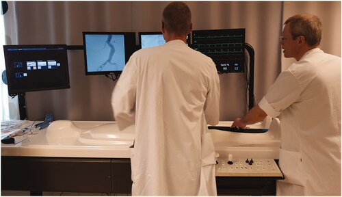
Figure 2. Patient with aneurysmal dilatation of the abdominal aorta, male, age 65. (A) Computed tomography angiography shows an aneurysm with a maximal diameter of 65 mm. (B) Segmented surface-rendered 3D reconstruction. (C) Detail from the STL model of the aortic bifurcation and the right common iliac artery. (D) The imported STL model (center) in the simulator stitched to the simulator template (light gray). (E) Angiogram of the stentgraft components on the simulator. (F) Angiogram of the stentgraft components in the patient. Visually E and F show good correlation. (G) CT-angiogram at six months follow-up.

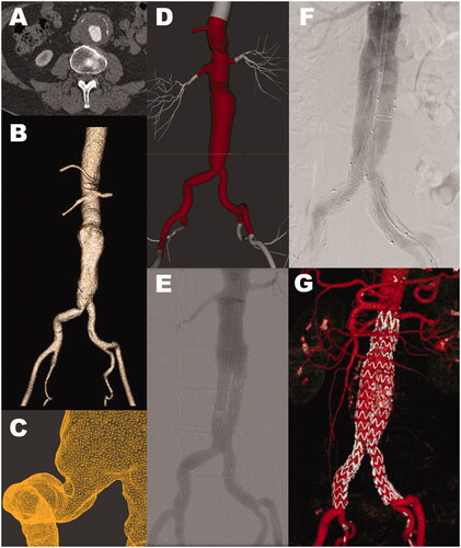
Figure 3. Patient with aneurysmal dilatation of the abdominal aorta, male, age 86 (A) Computed tomography angiography shows an aneurysm with a maximal diameter of 71 mm. (B) Segmented surface-rendered 3D reconstruction. (C) Detail from the STL model of the ostium of the artery to the left kidney. (D) The imported STL model (center) in the simulator stitched to the simulator template (light gray). (E) Angiogram of the stent-graft components on the simulator. (F) Angiogram of the stent-graft components in the patient. Visually E and F show poor correlation. (G) CT-angiogram at six months follow-up.

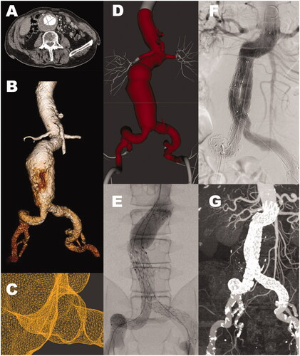
Figure 4. Comparing angiograms after stent graft deployment of four patients (I-IV) from the simulator (PsR) and from the real procedure (RP). Patient I, age 59, poor correlation; Patient II, age 82, good correlation; Patient III, age 63, poor correlation; Patient IV, age 80, good correlation. Stitching artefacts can be seen at the aortic neck of patient III and IV on the simulated pictures.

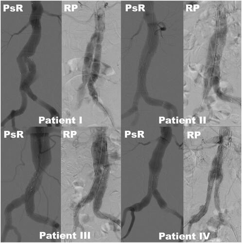
Figure 5. Boxplot presenting operator appraisal after the PsR on a Likert scale from 1 to 5, where 1 is disagree and 5 is strongly agree. N = 19. The middle band shows the median value, the bottom and the top of the boxes show the 25th and the 75th percentiles, and the ends of the whiskers show the 5th and the 95th percentiles. Outliers are plotted as circles and extreme outliers as stars.

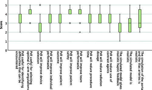
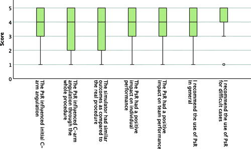
Figure 6. Boxplot presenting operator appraisal of seven statements after the procedure on a Likert scale from one to five, where one is disagree and five is strongly agree. N = 59. The middle band shows the median value, the bottom and the top of the boxes show the 25th and the 75th percentiles, and the ends of the whiskers show the 5th and the 95th percentiles. Outliers are plotted as circles.