Unstrained and strained flamelets for LES of premixed combustion

Figures & data

Figure 1. Typical variation of normalised filtered reaction rate in unstrained and strained flamelets.

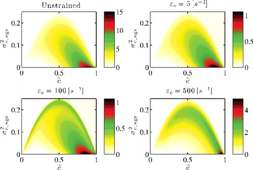
Figure 2. A schematic of the experimental [33] and computational setups of the validation case.

Figure 3. Comparison of measured [33] (symbols) and computed, using 1.5M (solid line) and 4.2M (dotted line) grids, normalised mean axial velocity and turbulent kinetic energy in the cold flow of flame F2.

Figure 4. Comparison of measured [33] (symbols) and computed (lines) radial variation of ⟨U⟩/U_b for the F1 and F3 flames. The unstrained flamelet result is shown for the 1.5M (

) and 4.2M (

) grids, and the strained flamelets result is shown for the 1.5M (

) and 4.2M (

) grids. The results for the 4.2M grid are shown only for the F1 flame.

Figure 5. Comparison of measured [33] (symbols) and computed (lines) radial variation of ⟨k⟩/k₀ for the F1 and F3 flames. See Figure 4 for legend.

Figure 6. The normalised mean temperature computed on the 1.5M grid using the UF (

) and SF (

) models is compared with measurements [33] (

). Previous results [7] (▵), [28] (), [32] (

) and [39] (

) are shown for comparison.

Figure 7. Comparison of measured [33] (

) and computed mean fuel mass fraction. The computational results are shown for the 1.5M grid using the UF (

) and SF (

) models. Previous results [7] (▵), [28] (), [32] (

) and [39] (

) are shown for comparison.

Figure 8. Spatial variation of in flame F3 obtained at an arbitrarily chosen time, t1, using (a) the UF and (b) the SF model with the 1.5M grid. These results at 20 ms later are shown in (c) and (d). The contours are shown for .

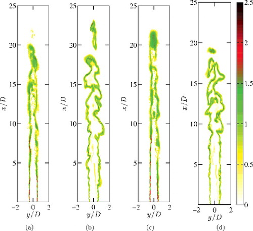
Figure 9. Spatial variation of in flame F1 obtained at an arbitrarily chosen time, t1, using (a) the UF and (b) the SF model with the 1.5M grid. These results at 20 ms later are shown in (c) and (d). The contours are shown for .

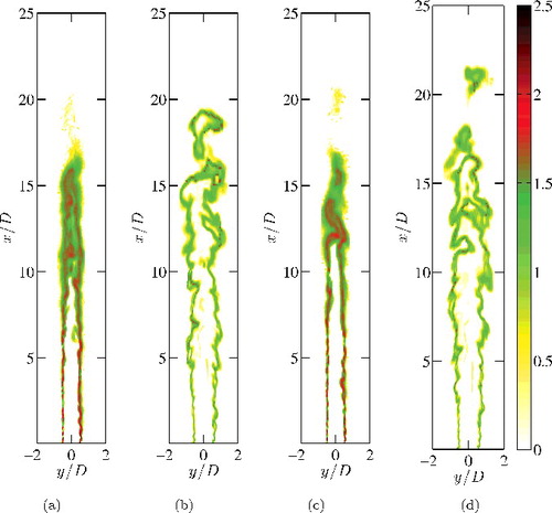
Figure 10. Comparison of measured [33] and computed mean mass fraction of H₂O. The legend is as shown in Figure 7.

Figure 11. Comparison of measured [33] and computed OH mass fractions. The legend is as shown in Figure 7.

Figure 12. Comparison of measured [33] and computed H₂ mean mass fractions. The legend is as shown in Figure 7.

Figure 13. PDFs of Da_Δ and Ka_Δ from flames F1 (top row) and F3 (bottom row). The results are shown for the UF (

) and the SF (

) models.

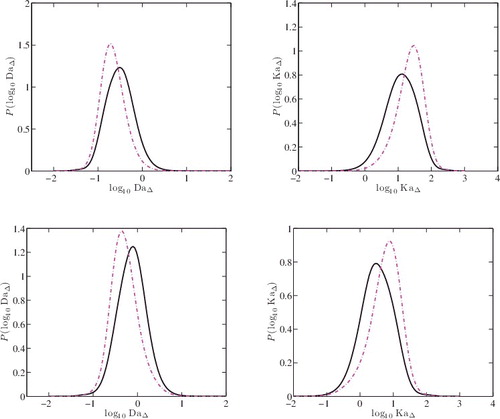
Figure 14. Scatter plot of computed σ²_{c, sgs} and its modelled value using with in the top row. The results for the revised model, with , are shown in the bottom row. The first and second columns are for the 1.5M and 4.2M grids of the F1 flame, respectively.

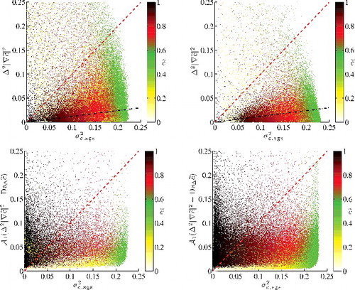
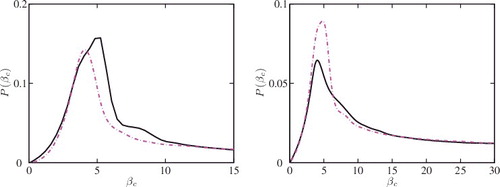
Figure 15. The PDF of β_c from (a) flame F1 and (b) flame F3 obtained using the UF (

) and SF (

) models with the 1.5M grid.

Y.C. Chen, N. Peters, G.A. Schneemann, N. Wruck, U. Renz, and M.S. Mansour, The detailed structure of highly stretched turbulent premixed methane–air flames, Combust. Flame 107 (1996), pp. 223–244.

 Web of Science ®Google Scholar

A. De and S. Acharya, Large eddy simulation of a premixed Bunsen flame using a modified thickened-flame model at two Reynolds numbers, Combust. Sci. Technol. 181 (2009), pp. 1231–1272.

 Web of Science ®Google Scholar

I.A. Dodoulas and S. Navarro-Martinez, Large eddy simulation of premixed turbulent flames using the probability density function approach, Flow Turbul. Combust. 90 (2013), pp. 645–678.

 Web of Science ®Google Scholar

H. Kolla and N. Swaminathan, Strained flamelets for turbulent premixed flames II: Laboratory flame results, Combust. Flame 157 (2010), pp. 1274–1289.

 Web of Science ®Google Scholar

G. Wang, M. Boileau, and D. Veynante, Implementation of a dynamic thickened flame model for large eddy simulations of turbulent premixed combustion, Combust. Flame 158 (2011), pp. 2199–2213.

 Web of Science ®Google Scholar