Figures & data
Table 1. Two eigenvalues with a smallest (non-zero) magnitude and the largest chemical components of the corresponding eigenvectors in chemical equilibrium.
Figure 1. A ribbon schematic representation of the 2D FGM-REDx for a part of the post-flame zone of a premixed flamelet. c-axis represents a scaled reaction progress variable. The remaining two axes show the mass fractions of CO and NO. The local directions of the eigenvectors and
are shown, respectively, in red and yellow. Grey are projections to ease the visualisation. This figure is available in colour online.
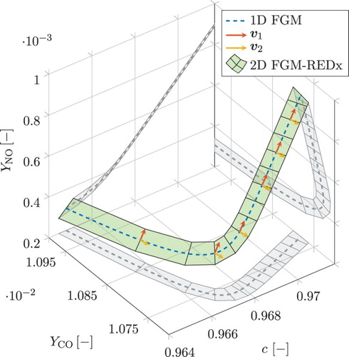
Figure 2. Magnitude of the projection of the unit vector tangent to the direction of the 1D FGM, , on the slowest eigenvector
(red) and the plane spanned by the two slowest eigenvectors,
(blue). This figure is available in colour online.
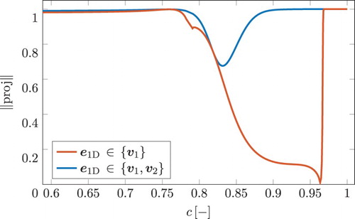
Figure 3. On the left side, an example is shown of the flat plane locally forming a 2D FGM-REDx for one grid point k. The plot regards a post-flame part of a premixed flamelet. Axes represent the progress variable, , a secondary reactive control variable,
, and the mass fraction of CO. The plot at the right, shows the tabulation grid for multiple grid points k on the 1D FGM in the plane of the two reactive control variables. This figure is available in colour online.

Figure 4. Flow diagram illustrating the procedure of the generation and tabulation of the -dimensional FGM-REDx, conditioned for one level of conserved control variables.
Table 2. Domain length L and the corresponding residence time τ for the series of the examined nozzle simulations.
Figure 5. Profiles of the surface area, Mach number, enthalpy and pressure in the NGV simulation.
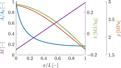
Table 3. Weights of chemical species in the definitions of the reactive control variables.
Figure 6. Tabulation grid for pressure (p) and enthalpy (h). Colour shows the local chemical equilibrium values for the mass fraction of CO. The red line shows the pressure and enthalpy curve of the expansion in an NGV simulation (from high pressure and enthalpy values to the low ones). This figure is available in colour online.
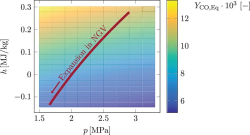
Figure 7. Schematic representation of the 2D FGM-REDx table grid of the two reactive control variables. Here the manifold is conditioned for one pressure and enthalpy level ( and h corresponds to
). The colour bar indicates the local CO mass fraction. The local chemical equilibrium point is given by the black dot. This figure is available in colour online.
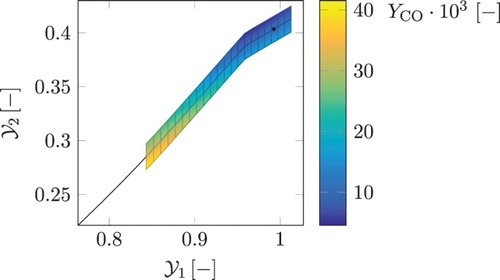
Figure 8. Detailed chemistry results (solid lines) and local chemical equilibrium (dashed line) for the mass fractions of CO and NO for various lengths of the domain: (corresponding to different residence times).
Figure 9. Reaction source term of CO for the three test simulations with the smallest residence times. Solid line represents the total source term. The values obtained considering only one chemical reaction, , are given by the blue dashdotted line. This Figure is available in colour online.
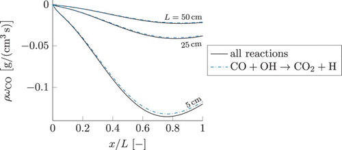
Figure 10. Chemical source terms of the local values of the two slowest eigenvectors and
postprocessed from the detailed chemistry simulation by taking an inner product of the species chemical source terms vector,
and the corresponding left eigenvector
. The source term magnitude is decreasing with incrementally increasing length of the domain L.
Figure 11. A priori FGM results for CO and NO. The two graphs on top correspond to the simulation case with the shortest residence time, the two at the bottom show the longest residence time case. The line styles for the results of the detailed chemical model (DC), local chemical equilibrium (Eq), the 1D FGM and the FGM-REDx are given in the legend. This figure is available in colour online.
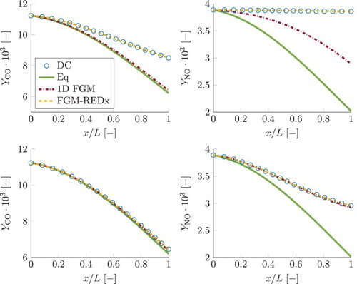
Figure 12. a priori FGM lookup for chemical source term of reaction progress variable. At the left plot simulation results are shown for the smallest residence time case, results shown at the right represent the simulation with the largest residence time. Legend for chemical models is similar to that in Figure . This figure is available in colour online.
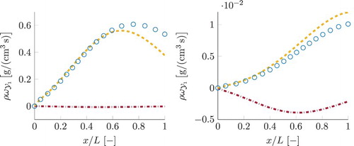
Figure 13. Simulation results for reaction progress variable, . Plot on the left represents the smallest residence time case, the one at the right represent the case with the largest residence time. Legend is similar to that in Figure . For 1D FGM and FGM-REDx, a posteriori results are shown. This figure is available in colour online.
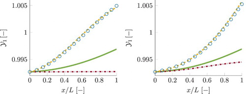
Figure 14. Simulation results for mass fractions of CO and NO. Line styles for different chemical models are given in the legend of Figure . The two subplots at the top correspond to the smallest residence time case, while the two at the bottom correspond to the case with the largest τ. This figure is available in colour online.
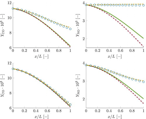
Figure 15. Surplus of the secondary reactive control variable, , compared to its local value in the 1D FGM,
. Detailed chemistry and FGM-REDx simulation results are shown using similar line styles as in Figure . Results for the case with the smallest τ are shown in the left subplot, the profiles for the case with the largest τ are shown in the right subplot. This figure is avaialble in colour online.
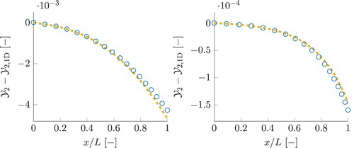
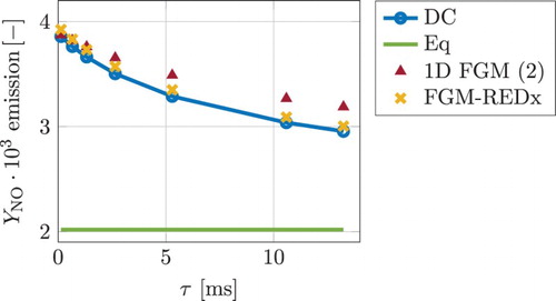
Figure 16. FGM predictions for CO emissions for multiple simulations plotted as function of the residence time τ. Line styles for detailed chemistry (DC), chemical equilibrium (Eq), 1D FGM and FGM-REDx are given in the legend. This figure is avaialble in colour online.
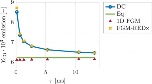
Figure 17. Results for the NO mass fraction (left) and the chemical source term (right) found applying various reduced modelling approaches. Detailed chemistry curve is used as the reference. Line styles representing detailed chemistry, local chemical equilibrium and the direct lookup values from the 1D FGM and the FGM-REDx are given in the legend of Figure . Purple lines show the 1D FGM results obtained by an additional NO transport equation, utilising various approaches for the source term modelling. Their corresponding line styles are given in the legend. This figure is available in colour online.
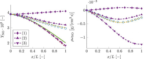
Figure 18. Values for the mass fraction of NO at the exhaust of multiple nozzle simulations with a varied domain length. Horizontal axis represents the residence time τ for each simulation. This figure is available in colour online.