A DNS assessment of linear relations between filtered reaction rate, flame surface density, and scalar dissipation rate in a weakly turbulent premixed flame

Figures & data

Figure. 1. Probability Density Function $P_2\left(R_2,\overline{c}\right)$ for a ratio of $R_2=\left(\mathrm{\nabla }\cdot \widehat{\rho D\mathrm{\nabla }c}+\hat{W}\right)/\left({\rho }_u{S}_L\widehat{|\mathrm{\nabla }c|}\right)$, obtained using Equation (10) at $\mathrm{\Delta }/{\delta }_L=1.15$ and various values of the Reynolds-averaged combustion progress variable $\overline{c}$, specified in legends.

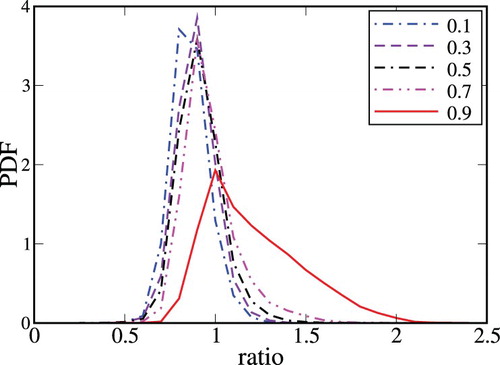
Figure 2. Probability Density Functions (a) $P_3\left(R_3,\overline{c}=0.5\right)$ and (b) $P_{\omega ,3}\left(\hat{\omega }=0.15\pm 0.005,R_3,\overline{c}=0.5\right)$ for a ratio of $R_3=\hat{W}/\widehat{\rho \chi }$. Different curves show results obtained using different normalised filter widths $\mathrm{\Delta }/{\delta }_L$, specified in legends.

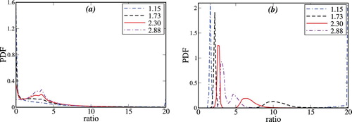
Figure 3. Reaction rate $W/{\rho }_u$ (red double-dashed-dotted line), FSD $S_L\mathrm{\nabla }c$ (black double-dotted-dashed line), SDR $\rho D\mathrm{\nabla }c\cdot \mathrm{\nabla }c/{\rho }_u$ (blue dotted-dashed line), and ratios of $W/\left({\rho }_u{S}_L\mathrm{\nabla }c\right)$ (black short-dashed line) and $W/\left(\rho D\mathrm{\nabla }c\cdot \mathrm{\nabla }c\right)$ (blue long-dashed line) vs. the normalised distance $\xi =x\text{max}\left\{|\mathrm{\nabla }c|\left(x\right)\right\}$ counted from the position of peak rate $W/{\rho }_u$ in the laminar flame that propagates from right to left.

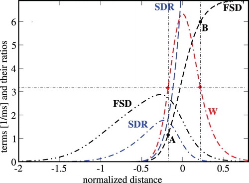
Figure 4. A 2D sketch of reaction zone (curve) and filter volumes.

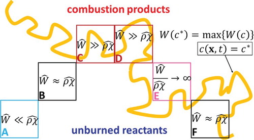
Figure 5. (a) Ratios $⟨R_3\text{|}\widehat{\rho c}/\hat{\rho }⟩=⟨\hat{W}/\widehat{\rho \chi }\text{|}\widehat{\rho c}/\hat{\rho }⟩$ (dotted-dashed and dotted lines) and $⟨R_4\text{|}\widehat{\rho c}/\hat{\rho }⟩=⟨\left(\mathrm{\nabla }\cdot \widehat{\rho D\mathrm{\nabla }c}+\hat{W}\right)/\widehat{\rho \chi }\text{|}\widehat{\rho c}/\hat{\rho }⟩$ (dashed and solid lines) conditioned to the filtered combustion progress variable $⟨\widehat{\rho c}/\hat{\rho }⟩$ and evaluated using various normalised filter widths $\mathrm{\Delta }/{\delta }_L$ specified in legends at the Reynolds-averaged combustion progress variable $\overline{c}=0.5$. (b) A ratio of $⟨R_2\text{|}\widehat{\rho c}/\hat{\rho }⟩=⟨\left(\mathrm{\nabla }\cdot \widehat{\rho D\mathrm{\nabla }c}+\hat{W}\right)/\left({\rho }_u{S}_L\hat{\mathrm{\Sigma }}\right)\text{|}\widehat{\rho c}/\hat{\rho }⟩$ conditioned to $⟨\widehat{\rho c}/\hat{\rho }⟩$ and evaluated using $\mathrm{\Delta }/{\delta }_L=1.15$ (solid and dashed lines) and 1.73 (dotted-dashed lines) at various values of the Reynolds-averaged combustion progress variable $\overline{c}$, specified in legends.

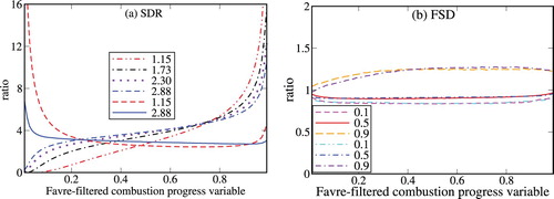
Figure 6. Mean reaction rate vs. Reynolds-averaged combustion progress variable $\overline{c}$. 1 – $\overline{\hat{W}}/{\rho }_u$. 2 – $2\overline{\widehat{\rho \chi }}/\left[{\rho }_u\left(2c_m-1\right)\right]$, where $c_m=0.88$ [27], 3 – $⟨R_3⟩\overline{\widehat{\rho \chi }}/{\rho }_u$, where the ratio $⟨R_3⟩=⟨\hat{W}/\widehat{\rho \chi }⟩$ is averaged over all cells characterised by $0.01<\hat{c}\left(\mathbf{\text{x}},t\right)<0.99$, 4 – $\overline{R_3}\overline{\widehat{\rho \chi }}/{\rho }_u$, where the ratio $\overline{R_3}\left(\overline{c}\right)$ is averaged over transverse plane provided that $0.01<\hat{c}\left(\mathbf{\text{x}},t\right)<0.99$. $\mathrm{\Delta }/{\delta }_L=2.88$.

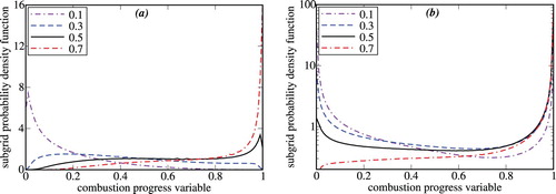
Figure 7. Subgrid conditioned PDFs $\hat{P}\left(c|\hat{c}\right)$ obtained at $\overline{c}=0.5$ and (a) $\mathrm{\Delta }/{\delta }_L=1.15$ or (b) $\mathrm{\Delta }/{\delta }_L=2.88$. Note that the PDFs are shown in linear and logarithmic scales in (a) and (b), respectively. The PDF sampling was performed for all grid points within a filter volume centred around a point $\mathbf{\text{x}}$ at instant $t$, followed by averaging the PDFs $P\left(c,\mathbf{\text{x}},t\right)$ for all $\mathbf{\text{x}}$ and $t$ such that ${\hat{c}}^{\ast }+0.005\le \hat{c}\left(\mathbf{\text{x}},t\right)<{\hat{c}}^{\ast }+0.005$. Values of ${\hat{c}}^{\ast }$ are specified in legends.

A.N. Lipatnikov, S. Nishiki, and T. Hasegawa, DNS assessment of relation between mean reaction and scalar dissipation rates in the flamelet regime of premixed turbulent combustion, Combust. Theory Modell. 19 (2015), pp. 309–328. doi: 10.1080/13647830.2015.1021837

 Web of Science ®Google Scholar