A super-grid approach for LES combustion closure using the Linear Eddy Model

Figures & data

Figure 1. Triplet map approximates the stirring effect of a single turnover of an isotropic turbulent Eddy; the coloured lines are concentration isopleths for a scalar; the figure on the left represents a scalar gradient where the straight line shows concentration.

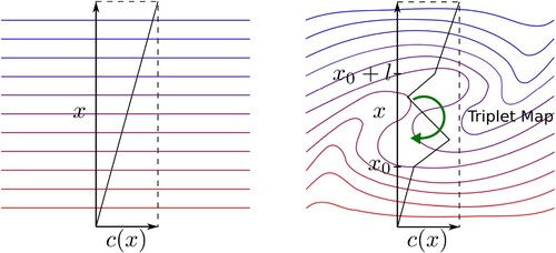
Figure 2. Schematic representation of SG-LEM. LEM line widths are smaller than implied by Equation (20(20) $A=\frac{\left(\sum _{j\in \mathbf{V}}{V}_j\right)}{l_t}.$(20) ).

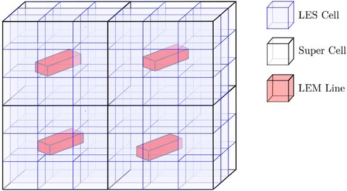
Figure 3. Schematic showing flux ordered splicing; arrows of different length indicate unequal fluxes between cells or cell clusters.

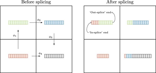
Figure 4. Interface between LES, super-grid and LEM.

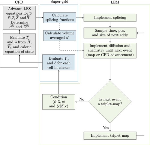
Figure 5. Numerical setup for the test case. (a) The computational domain. $H=1.466\mathrm{c}\mathrm{m}$ and $D=0.3048\mathrm{c}\mathrm{m}$, spanwise width is $1\mathrm{c}\mathrm{m}$ and (b) LES mesh.

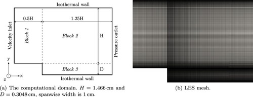
Figure 6. Top row: snapshots of Favre averaged progress variable c at the LEM level; bottom row: LES resolved $\tilde{c}$ as advanced by Equation (27(27) $\frac{\mathrm{\partial }\left(\overline{\rho }\tilde{c}\right)}{\mathrm{\partial }t}+\mathrm{\nabla }\cdot \left(\overline{\rho }\tilde{\mathbf{u}}\tilde{c}\right)=\mathrm{\nabla }\cdot \left[\frac{{\mu }_t}{S{c}_t}\mathrm{\nabla }\tilde{c}\right]+\overline{\rho }\tilde{\dot{c}},$(27) ) at different times; scalars imaged at $z=0.5\mathrm{c}\mathrm{m}$; 125 CFD cells per cluster.

Figure 7. Row I: snapshots of Favre averaged T the LEM level; row II: LES resolved $\tilde{T}$ as advanced by Equation (5(5) $\frac{\mathrm{\partial }\left(\overline{\rho }\tilde{H}\right)}{\mathrm{\partial }t}+\frac{\mathrm{\partial }\overline{\rho }{\tilde{u}}_j\tilde{H}}{\mathrm{\partial }{x}_j}={\tilde{u}}_j\frac{\mathrm{\partial }\overline{p}}{\mathrm{\partial }{x}_j}+\frac{\mathrm{\partial }}{\mathrm{\partial }{x}_j}\left({\alpha }_{\mathrm{E}\mathrm{f}\mathrm{f}}\frac{\mathrm{\partial }\tilde{H}}{\mathrm{\partial }{x}_j}\right)+\frac{\mathrm{\partial }p}{\mathrm{\partial }t}.$(5) ) along with (7(7) $\tilde{H}=\sum _{\alpha =1}^N{\tilde{Y}}_{\alpha }\times \left(h_{\alpha }\right(T)+h_{\alpha }^0),$(7) ); row III: LES resolved $\tilde{T}$ as advanced by Equation (25(25) $\tilde{\psi }(\mathbf{x},t)={\int }_0^1〈\psi |Z,c〉P\left(Z\right)P\left(c\right)\mathrm{d}Z\mathrm{d}c.$(25) ) for corresponding times (units [K]). Scalars imaged at $z=0.5\mathrm{c}\mathrm{m}$.

Figure 8. Top row: snapshots of Favre averaged $Y_{{\mathrm{C}\mathrm{O}}_2}$ at the LEM level; bottom row: LES resolved ${\tilde{Y}}_{{\mathrm{C}\mathrm{O}}_2}$ as advanced by Equation (25(25) $\tilde{\psi }(\mathbf{x},t)={\int }_0^1〈\psi |Z,c〉P\left(Z\right)P\left(c\right)\mathrm{d}Z\mathrm{d}c.$(25) ) for corresponding times. Scalars imaged at $z=0.5\mathrm{c}\mathrm{m}$.

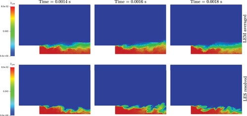
Figure 9. Top row: Favre averaged $\mathrm{O}\mathrm{H}$ mass fractions for each LEM line; bottom row: LES resolved $\mathrm{O}\mathrm{H}$ mass fractions using Equation (25(25) $\tilde{\psi }(\mathbf{x},t)={\int }_0^1〈\psi |Z,c〉P\left(Z\right)P\left(c\right)\mathrm{d}Z\mathrm{d}c.$(25) ).

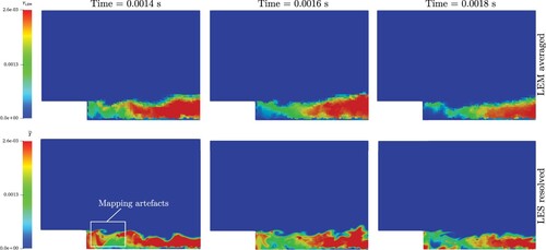
Figure 10. Mean velocity $U_x$ profiles.

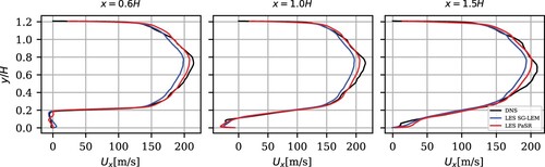
Figure 11. Mean temperature profiles.

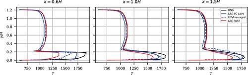
Figure 12. Mean mass fractions.

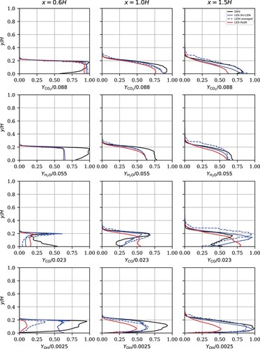
Figure 13. Species reaction rates, scaled [$\mathrm{k}\mathrm{m}\mathrm{o}\mathrm{l}{\mathrm{m}}^{-3}{\mathrm{s}}^{-1}$].

Figure 14. Top row: snapshots of Favre averaged c at the LEM level; bottom row: LES resolved $\tilde{c}$ for corresponding times. Scalars imaged at $z=0.5\mathrm{c}\mathrm{m}$. 1000 CFD cells per cluster.

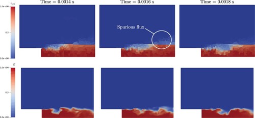
Figure 15. Mean c profiles, comparing cluster sizes of 125 and 1000.

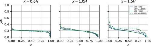
Figure 16. Mean profiles for radical mass fractions, cluster size of 1000.

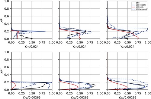
Table 1. Performance comparison.

#	Combustion closure	Time (h)
1	PaSR	108
2	SG-LEM125	50
3	SG-LEM1000	40
4	LES–LEM	969 (estimated)

Note: Numbers in curly brackets indicate number of CFD cells per cell-cluster.All simulations used a grid size of 6.2 M cells and 256 processors.