The São Paulo wholesale seafood market: A study of fish prices in Brazil

Figures & data

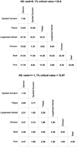
Figure 1. Apparent seafood consumption per capita per year in Brazil, and its components (domestic production from capture and aquaculture, imports, and exports) from 2000 to 2020. Apparent consumption per capita is defined as production (from aquaculture and fisheries) plus imports minus exports, divided by population. Source: FAO (2021) ans Seafood Brasil (2021).

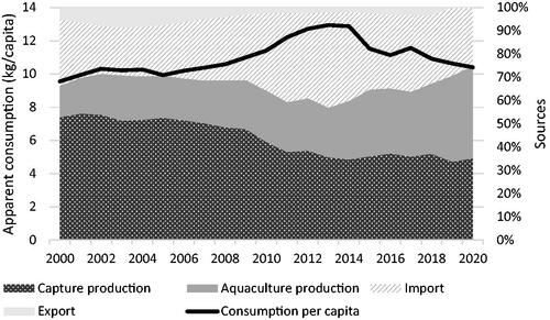
Table 1. Descriptive statistics of fish and meat prices.

Species	Mean ($R/kg)	C.V. (%)^a	Volatility (%)^b	Mode	Production	Type	Stationary^d
Common snook	33.40	10.9	9.9	Fishery	Domestic	Whitefish	TS
Flatfish	12.35	15.5	10.8	Fishery	Domestic	Whitefish	TS
Mullets	6.85	22.2	16.0	Fishery	Domestic	Whitefish	TS
Sardine	4.70	39.2	26.0	Fishery	Domestic/Imports	Small Pelagic	TS
Spanish mackerel	9.93	14.1	12.8	Fishery	Domestic	Pelagic	TS
Shark	8.70	13.1	7.1	Fishery	Domestic/Imports	Whitefish	TS
Skipjack	2.92	15.2	13.4	Fishery	Domestic	Pelagic	TS
Weakfish	9.14	12.5	10.3	Fishery	Domestic	Whitefish	TS
Whitemouth croaker	4.76	21.9	14.2	Fishery	Domestic	Whitefish	TS
Codling	5.15	25.0	14.1	Fishery	Domestic	Whitefish	TS
Amberjack	21.52	13.3	15.1	Fishery	Domestic	Pelagic	TS
Perch	17.60	13.3	14.6	Fishery	Domestic	Whitefish	TS
Yellowtail	14.60	22.0	22.2	Fishery	Domestic	Pelagic	TS
Salmon	28.59	23.6	7.8	Aquaculture	Imports	Salmonide	NS
Spotted sorubim	11.81	14.7	4.6	Aquaculture	Domestic	Whitefish	NS
Tilapia	5.90	21.4	6.2	Aquaculture	Domestic	Whitefish	NS
Largehead hairtail^c	4.07	23.4	12.2	Fishery	Domestic	Pelagic	NS
Chicken	4.23	23.4	6.7	–	–	–	NS
Beef	11.03	31.8	3.7	–	–	–	NS
Pork	4.49	30.0	10.1	–	–	–	NS

Note: ^aC.V. is the coefficient of variation, the standard deviation of the price divided by the mean price. ^bVolatility is the standard deviation of monthly logarithmic price returns. ^cLargehead Hairtail shows a mixed result for unit-root tests, a borderline non-statiotionary/trend-stationary case. ^dStationary refers to whether the price is classified as trend-stationary or non-stationary based on the results in Table 2.

Figure 2. Monthly fish and meat price indices for São Paulo August 2013 to July 2021. Source: CEAGESP (2021) and CEPEA (2021).

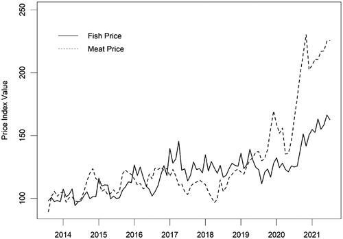
Table 2. Unit root test statistics.

	ADF statistic	ERS statistic	PP statistic
5% Critical value	−2.49	−3.03	p-Values
Common snook	−5.53	−5.46	<0.010
Flatfish	−4.60	−4.58	<0.010
Mullets	−4.14	−4.12	<0.010
Salmon	−2.65	−2.74	0.346
Sardine	−4.88	−4.03	<0.010
Spanish mackerel	−4.72	−4.48	<0.010
Shark	−4.55	−3.95	<0.010
Spotted sorubim	−1.09	−1.03	0.737
Tilapia	−2.14	−2.17	0.535
Skipjack	−4.98	−4.12	<0.010
Weakfish	−3.55	−3.54	<0.010
Whitemouth croaker	−3.79	−3.30	<0.010
Codling	−3.85	−3.78	<0.010
Amberjack	−4.53	−4.50	<0.010
Largehead hairtail	−2.86	−2.77	<0.017
Perch	−5.30	−5.33	<0.010
Yellowtail	−5.13	−5.00	<0.010
Chicken	−2.53	−2.73	0.529
Beef	−0.60	−1.00	0.982
Pork	−2.49	−2.54	0.259

Note: Null hypothesis is a unit-root, stochastic trend. Alternative hypothesis implies linear trend stationary prices. Lag order selected according to the AIC. The ADF and ERS statistics show test statistics with associated 5% critical values at the top row. The PP test reports p-values for the null hypothesis.

Figure 3. Significant (p-value < 0.01) correlations in monthly logarithmic price changes.

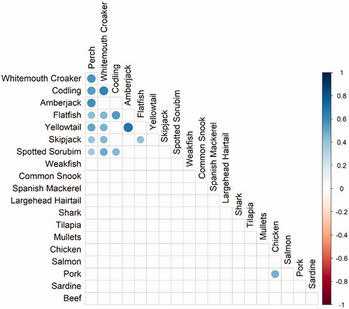
Figure 4. Significant (p-value < 0.01) price level correlations among stationary fish prices. Significance evaluated using Newey West standard errors.

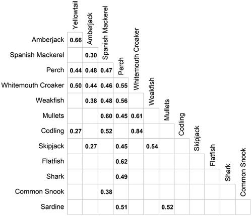
Figure 5. Trace test statistics for the rank of the bivariate cointegration matrix. A stable price relationship requires rejection of the first H₀: r = 0 but non-rejection of H₀: r < = 1, implying a common stochastic price trend. Specification assumes unrestricted constant, and lag order of the VAR testing equation selected according to the AIC with a maximum lag of 6 months.

FAO. (2021). Aquaculture production 1950-2019. Universal Software for Fishery Statistical Time Series.

 Google Scholar

Seafood Brasil. (2021). Você sabe quanto o brasileiro realmente come de pescado? Seafood Brasil, 9.

 Google Scholar

CEAGESP (Companhia de Entrepostos e Armazéns Gerais de São Paulo). (2021). CEAGESP (Companhia de Entrepostos e Armazéns Gerais de São Paulo). Pescado. http://www.ceagesp.gov.br/entrepostos/pescado/

 Google Scholar

CEPEA. (2021). Agricultural prices. https://www.cepea.esalq.usp.br/br

 Google Scholar