Figures & data
Figure 1. Distribution of the selected meteorological stations in the study area. The number between brackets after each station represents its unique ID.
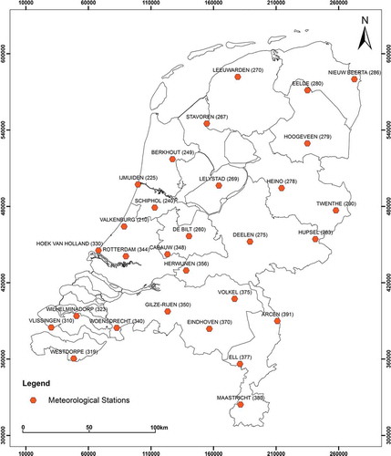
Figure 2. The four phases of the analytical workflow for interactively discover wind characteristics.
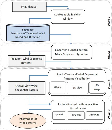
Figure 3. (a) The new IDs (itemsets) generated from the combination of wind speed and direction IDs, (b) the sliding window that moves along the list of itemsets according to the length_range (48) and step_v (24) parameter values, and (c) sequence database that consists of transactions (window 1, 2,…, n) and each transaction gets assigned a unique ID (TID).
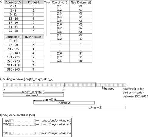
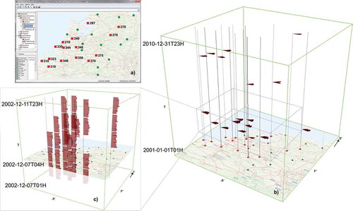
Figure 4. The interactive visualization tools used for wind pattern exploration: (a) overall view of the frequent wind sequential patterns in TileVis, (a1) a magnified view of the axes of TileVis, (b) a 3D view (STC) that allows visualizing wind speed and direction, (b1) A magnified view of one of the wind roses illustrated in the STC, and (c) a 2D map to show the stations that contain the patterns selected in TileVis.
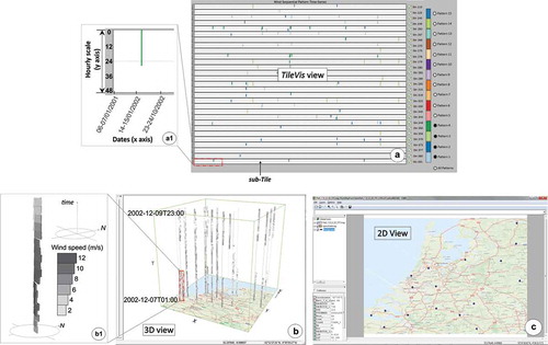
Figure 5. (a) TileVis visualization for overall wind sequential patterns distribution, (b) distribution of wind sequential patterns for stations 255, 240 and 249 in TileVis, (c) focusing wind patterns in selected time moment (from 25 to 30 December 2008), and (d) distribution of pattern 12 in all stations for the whole period of study.
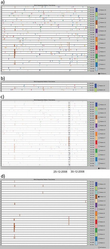
Figure 6. Visual representation of wind sequential patterns using 3D wind rose (P = pattern, L = length and F = frequency). Each of the 3D wind rose based is referred to pattern colours (refer to ).
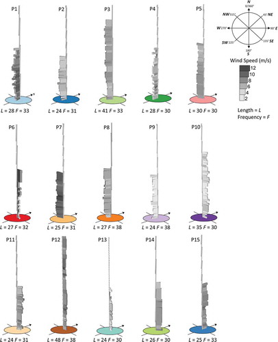
Figure 7. Wind sequential patterns illustrated using 3D wind roses and coloured according to (a) the type of pattern, and (b) to their speed (m/s).
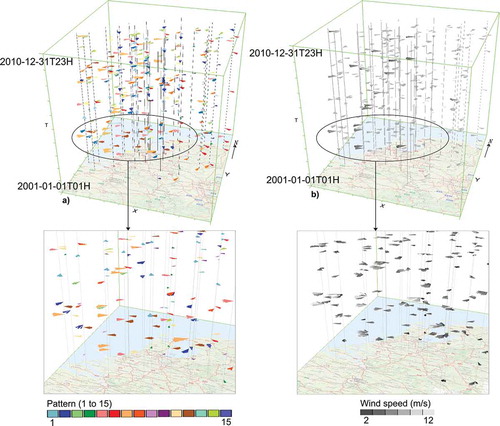
Figure 8. Wind sequential patterns in 3D view and 2D map: (a) the 2D map shows the positions of the selected stations highlighted in square symbol, and (b) occurring wind sequential patterns over time which visualized on top of the stations.
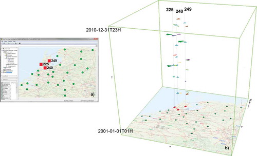
Figure 9. Wind sequential pattern occurrences during the selected time interval: (a) highlighted stations indicate stations that contain at least one of the selected patterns, (b) wind sequential patterns occurrences in time with different patterns in STC, and (c) visualizing wind speed and direction for reoccurring pattern 11 (red dot line).
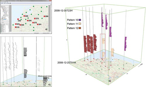
Figure 10. Similar wind pattern occurrences: (a) 2D map highlights the stations that contain pattern 12 with square symbol (red colour), (b) distribution of pattern 12 for the whole period of study, and (c) reoccurring pattern 12 in the selected time period (blue dot box in 10b).