Figures & data
Figure 1. By applying a split operator, a polygon can be fairly distributed among its neighbours. (a) Polygon to be split. (b) New boundaries. (c) Result of split operation.
Figure 2. Requirements for our split operation (area object to be split is shown in grey). Circled numbers are the attractiveness values of the neighbours. (a) Larger pieces should be assigned to more attractive neighbours. (b) Certain neighbours should be prevented from getting a share. (c) Resulting line work should fit in and connect to the remaining boundaries. (d) Input features might have holes and splitting should take these holes (containing another feature) in consideration.
Figure 3. An example showing SPLITAREA at work. (a) The splittee: the object that has to be subdivided over its neighbours. (b) The perimeter chains (labelled a, b, c) and the three external chains (chains incident with the perimeter chains). (c) Inside the splittee, skeleton edges will be created. The new boundaries will be formed by these edges and the external chains.
Figure 4. Selection of internal triangles. (a) Walk on internal triangles. (b) Triangulation of the splittee, where all internal triangles have been selected. Also external chains are shown.
Figure 5. Four types of triangles can be distinguished by looking at the number of G-edges: 0-triangles, 1-triangles, 2-triangles and 3-triangles. By connecting the midpoints of the D-edges (unconstrained edges), a skeleton edge can be obtained (skeleton edges are visualized with dashed lines).
Figure 6. Creation of the skeleton. (a) Obtaining skeleton edges using the triangulation. Note: triangle type is indicated by grey tone (cf. ). (b) Adding extra skeleton edges (connectors) to guarantee a connection between the existing external chains (those need to be preserved) and the skeleton. Note that a connector has to be chosen for the node touching the external chain at the top right.
Figure 7. Connectors are created if a corner vertex of a triangle also is a node in the planar partition (skeleton edges are visualized with dashed lines). (a) The four different triangle types and how connectors are generated per type. (b) Skeleton edges and connectors are created locally (depending on triangle type) and duplicate connectors for neighbouring triangles are avoided.
Figure 8. Labelling the skeleton edges with the correct neighbour reference and pruning parts of the skeleton that are enclosed completely by one neighbour. (a) All skeleton edges created (dashed, inside the splittee) and the external chains (dark grey). (b) Labelling of the created skeleton edges (light grey), starting from an external chain (dark grey). Note: edges that have the same neighbouring reference value on both sides once labelled are drawn in black. (c) Parts of the graph that have the same label on both sides (black) are removed. Shortcuts (dashed) replace the two skeleton edges that touch the branches that are removed.
Figure 9. Result obtained with SPLITAREA (a) All skeleton edges and external chains are merged into the longest topological chains possible (having the same neighbour references). (b) The line work obtained fits in with the rest of the planar partition.
Figure 10. Handling islands when splitting a face (face A). No extra steps have to be taken for label propagation when a hole is filled by more than one face (cf. faces E and F). However, care has to be taken when holes are filled by only one face (face B), or when island faces are tangent in one node (faces C and D). (a) Careful labelling is necessary when handling islands. (b) Result.
Figure 11. Weights are set on the perimeter chains and are entered in the triangulation at the vertices. The new vertices of the skeleton edges are moved along the unconstrained triangulation edge accordingly. The vertices where the external chains are incident have two weights set.
Figure 12. Fixing the border of the domain can be performed with zero weights.
Figure 13. Triangles with zero-weight vertices. Unmovable vertices, having a weight = 0, are coloured grey. Skeleton segments that will be created are in black, skeleton segments that will not be created are visualized with grey (e.g. triangle type-0-2-vertices).
Figure 14. Fixed perimeter chains (i.e. zero-weight vertices) bring some special implications. This is illustrated with two cases. (a) Zero-weight edges can lead to cycles (corresponding to neighbour y, with fixed boundary) in the skeleton graph. The labelling step thus should be modified such that neighbour x gets the complete area of the splittee. (b) Also with zero-weight vertices, triangles are processed locally (independent of all other triangles). However, more possibilities have to be taken into account (cf. ). Note that triangles that have a zero-weight vertex have their constraints visualized in black and are labelled with their position in .
Table 1. Characteristics of the test data sets used in the experiments.
Figure 15. Clips from both test data sets. German land-cover data set. (b) European land-cover data set.
Figure 16. Results of first, unweighted run of SplitArea. (a) Histogram of the errors occurring while splitting faces. An error is the difference between the expected and actual share obtained by a neighbouring face. (b) Distribution of the errors over the domain. The larger and darker a circle is, the larger the total error in the outcome of the performed split is.
Figure 17. (a) & (b): Face A completely surrounds the splittee and gobbles it up. (c) & (d): On the boundary of the splittee, the vertices are distributed unevenly, leading to small triangles in front of face A: these triangles prevent face A from getting its balanced share of the splittee. (a) Completely surrounded splittee, face A gets all of the splittee. (b) Improved split. (c) Unevenly distributed vertices prevent face A from getting a share. (d) Improved split.
Figure 18. Results of a weighted run of SplitArea, using zero weights (with simplification and densification) to fixate the border of the domain. (a) Total errors made. (b) Distribution of errors over the domain. Errors at the border of the domain have been solved.
Figure 19. Comparing the straight skeleton, splitting the face of , with the result of SplitArea. Whereas with SplitArea it is usually necessary to add additional connectors (cf. ), the straight skeleton has connectors to all vertices and all unwanted branches need to be pruned. (a) Split using straight skeleton, including all branches. (b) Straight skeleton after pruning. (c) Split using SPLITAREA.
Figure 20. SplitArea versus straight skeleton after 480 splits. Note that in this case, no densification or line simplification has been applied. (a) German land-cover data set. (b) SPLITAREA. (c) Straight skeleton.
Table 2. Empirical results: comparing merge operation with split operation.
Figure 21. A series of maps derived from the tGAP structure. The series illustrate the (subtle) differences between the merge and split operations. Note that the maps with lesser areas should be drawn smaller and smaller. (a) Most detailed representation of European land-cover data set (1590 areas). The circles indicate regions where the merge and split approaches give notable different result. (b) Merge I (360 areas remaining). (c) Split I (360 areas remaining). (d) Merge II (120 areas remaining). (e) Split II (120 areas remaining). (f) Merge III (60 areas remaining). (g) Split III (60 areas remaining).
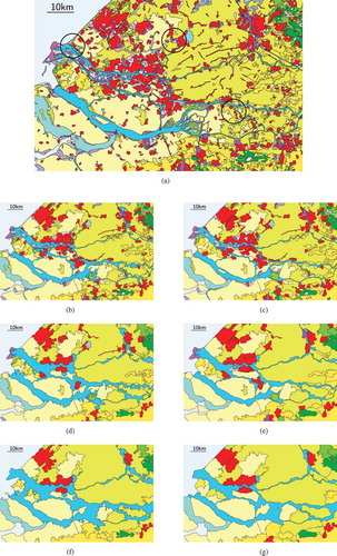
Figure 22. Influence of connector for fair split: weighted skeleton shown within splittee with dotted lines (fair based on weights at opposite site of splittee) and current connector depicted with short dashed line. A better connector, depicted with the long dashed line (based on the weights of adjacent neighbours at same side of the splittee).
Figure 23. Alternative application of SplitArea: horizontal conflation. Two cross-border data sets have gaps (white areas) between them. SplitArea can be used to split those gaps. Figure taken from Ledoux and Arroyo Ohori (Citation2011).