
Figures & data
Table 1. A list of all datasets, sources and descriptions used in our case study.
Table 2. Example restrictions to road networks from OSM labels.
Table 3. The values for each distance metric compared with actual road distance and travel time matrices.
Table 4. Selected hyperparameters for all experiments (1)–(6) (Exp. 1–6) with dead-zone 10-fold cross-validation.
Table 5. Results from four validation techniques: 10-fold cross-validation, spatially stratified 10-fold cross-validation, chequerboard holdout and spatial dead-zone 10-fold cross-validation.
Figure 1. A comparison of the actual road, Euclidean, Minkowski and Manhattan distances between two points on a map (OpenStreetMap Contributors Citation2008).
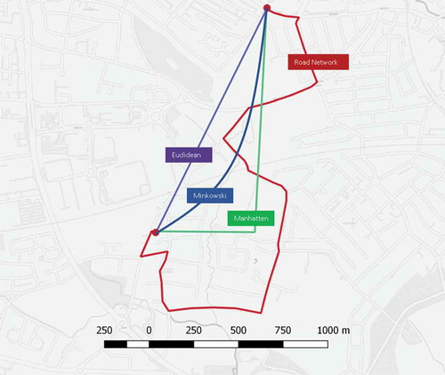
Figure 2. Illustration of the spatial transformation from road distance (or travel time) into a Euclidean space.
Figure 3. A flow diagram diagrammatically depicting the entire experimental process for the UK real-estate valuation case study described in this paper.
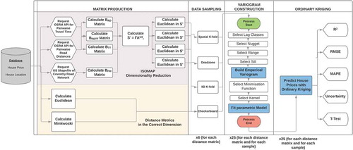
Figure 4. A plot of all locations and prices in the houses dataset. Small and light points represent cheaper houses and large dark points represent the more expensive.
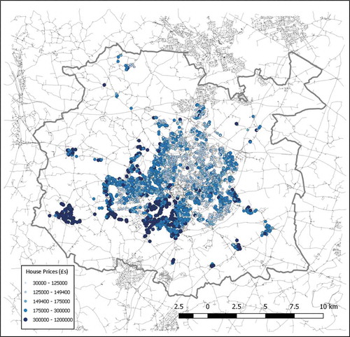
Figure 5. A comparison of all sampling techniques: (a) chequerboard holdout: training points (black grid) and testing points (white grid); (b) spatial k-fold with dead-zone radii: yellow points are removed from the training set; (c) blue points are the training set and brown points are the test set, spatial K = 1; (d) blue points are the training set and brown points are the test set, spatial K = 2; (e) blue points are the training set and brown points are the test set, standard K = 1; and (f) blue points are the training set and brown points are the test set, standard K = 2.
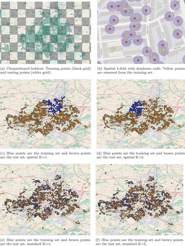
Figure 6. A graph of the three best kernels for a road distance matrix.
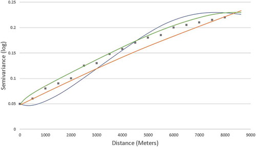
Table 6. Maximum likelihood results with dead zone spatial k-fold cross-validation.
Table 7. A comparison of the results from Crosby et al. (Citation2018) with those from this research using 10-fold cross-validation.