Spatio-temporal regression kriging for modelling urban NO₂ concentrations

Figures & data

Figure 1. Locations of the airboxes in Eindhoven which were used for this study. The black line represents the municipal boundary. The coloured lines represent major roads.

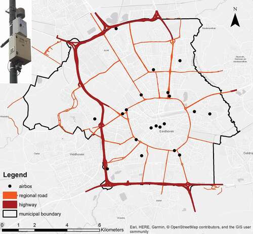
Table 1. $\hat{\beta }$ and p-values for the trend part of the regression model. The baseline for road type is ‘no road’. The baseline wind direction is ‘calm/variable’, the baseline weekday/weekends is ‘weekday’, and the baseline for hour is ‘0ʹ (23:00–0:00).

Covariate	Covariate unit	$\hat{\beta }$	p-value
Intercept	N/A	−113.38	<0.001
Population density	Inhabitants km^−2 (x1000)	1.47	<0.001
Road type: Small roads	Factor	0.59	0.02
Road type: Main roads	Factor	16.16	<0.001
Easting	km	0.82	<0.001
Relative humidity	%	−0.07	<0.001
Wind speed	m s^−1	−1.03	<0.001
Wind dir.: North	Factor	−2.11	<0.001
Wind dir.: North-East	Factor	−2.00	<0.001
Wind dir.: East	Factor	−4.23	<0.001
Wind dir.: South-East	Factor	−2.67	<0.001
Wind dir.: South	Factor	−1.76	<0.001
Wind dir.: South-West	Factor	0.19	0.71
Wind dir.: West	Factor	−0.92	0.10
Wind dir.: North-West	Factor	−1.28	0.07
Weekday: Weekend	Factor	−3.79	<0.001
Hour: 1	Factor	−1.61	0.004
Hour: 2	Factor	−2.25	<0.001
Hour: 3	Factor	−2.97	<0.001
Hour: 4	Factor	−3.20	<0.001
Hour: 5	Factor	−2.77	<0.001
Hour: 6	Factor	−0.50	0.37
Hour: 7	Factor	2.59	<0.001
Hour: 8	Factor	3.91	<0.001
Hour: 9	Factor	3.29	<0.001
Hour: 10	Factor	2.59	<0.001
Hour: 11	Factor	2.04	<0.001
Hour: 12	Factor	2.14	<0.001
Hour: 13	Factor	2.78	<0.001
Hour: 14	Factor	4.32	<0.001
Hour: 15	Factor	6.03	<0.001
Hour: 16	Factor	8.05	<0.001
Hour: 17	Factor	9.70	<0.001
Hour: 18	Factor	8.99	<0.001
Hour: 19	Factor	6.78	<0.001
Hour: 20	Factor	5.46	<0.001
Hour: 21	Factor	4.68	<0.001
Hour: 22	Factor	4.36	<0.001
Hour: 23	Factor	2.70	<0.001

Figure 2. Spatio-temporal sample variogram (left) and sum-metric fitted variogram model (right).

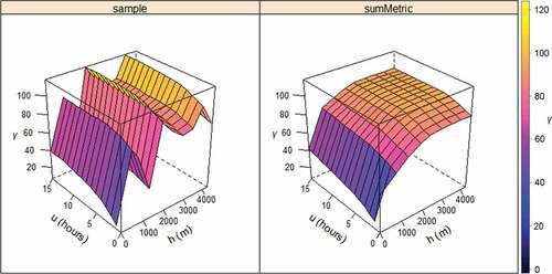
Table 2. Spatio-temporal variogram parameter estimates for the fitted sum-metric variogram.

Parameter	Estimate
${\tau }_s^2$	35.2 (µg m^−3)^2
${\sigma }_s^2$	0.00 (µg m^−3)^2
${\varphi }_s$	2692 m
${\tau }_t^2$	0.00 (µg m^−3)^2
${\sigma }_t^2$	10.8 (µg m^−3)^2
${\varphi }_t$	6.1 hrs
${\tau }_{joint}^2$	10.6 (µg m^−3)^2
${\sigma }_{joint}^2$	40.3 (µg m^−3)^2
${\varphi }_{joint}$	2670 m
$\kappa$	61.1 m hr^−1

Figure 3. Prediction maps of NO₂ concentrations at four time stamps on Monday the 7th of November, 2016 (UTC time; local time is 1 hour later). The covariate ‘population density’ was included as lattice data, creating clearly distinguished features for the neighborhoods. The red ellipse indicates a hotspot, with locally elevated NO₂ concentrations around the southern main city entrance road.

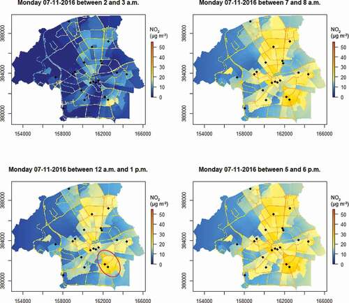
Figure 4. Prediction maps of NO₂ concentrations at four Sundays in November 2016, between 5 and 6 p.m. (UTC time; local time is 1 hour later). Note that different concentration limits were used as compared to Figure 3, to visualize the high concentrations on the 27th of November.

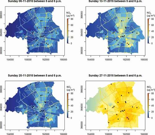
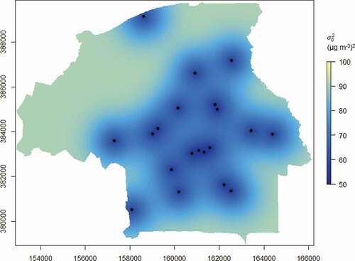
Figure 5. Kriging variance map (Monday 07-11-2016 between 7 and 8 a.m.).

Data and codes availability statement

The data and codes that support the findings of this study are available in DANS with the identifier 10.17026/dans-xmp-fw6h.