Figures & data
Figure 1. (a) A 100-by-100 raster surface consisting of 10 different classes, to which two sets of cost values, 1 to 10 and 11 to 20, are assigned. Note that darker cells have higher cost values. (b) Two least-cost paths between two terminal cells (circled) on the cost surface with the different sets of values. The path generated with the cost values of 1 to 10 (lightly shaded) deviates from that with the cost values of 11 to 20 (darkly shaded)
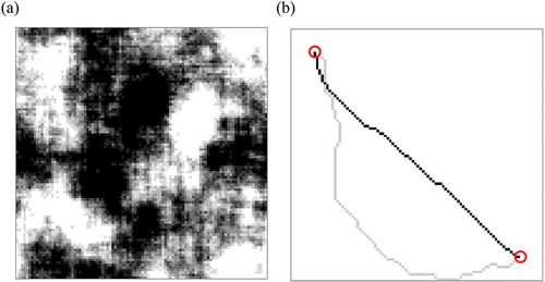
Figure 2. Examples of (a) and (b) cloudy cost surfaces and (c) and (d) patchy cost surfaces. Note that darker shades represent higher values
Figure 3. (a) a minisum-cost path (enclosed by bold lines) and (b) a minimax-cost path (shaded) in a raster cost surface. Note that the number in each cell represents the cost value assigned to that cell
Figure 4. (a) a minisum-unsuitability path (enclosed by bold lines) and (b) a maximin-suitability path (shaded) in a raster suitability surface. Note that the number in each cell represents the suitability value assigned to that cell
Table 1. Results of experiment 1 corresponding to the first 10 pairs of a minisum-cost path and minimax-cost path generated (a) on cloudy cost surfaces and (b) on patchy cost surfaces
Figure 5. Frequency distributions of l(minimax)/l(minisum) (a) on cloudy cost surfaces and (b) on patchy cost surfaces
Figure 6. Frequency distributions of u(minisum)/u(minimax) (a) on cloudy cost surfaces and (b) on patchy cost surfaces
Table 2. Numbers of cases in which minimax-cost paths performed better than (1st column), equal to (2nd column), or worse than (3rd column) their paired minimum-cost path with respect to the maximum, 75th percentile, 50th percentile, 25th percentile, or minimum-cost value (a) on cloudy cost surfaces and (b) on patchy cost surfaces. (a) On cloudy cost surfaces (b) On patchy cost surfaces
Figure 7. Frequency distributions of the ratio of the mean-suitability length of a maximin-suitability path to that of its paired minisum-unsuitability path (a) on cloudy suitability surfaces and (b) on patchy suitability surfaces
Figure 8. Frequency distributions of the ratio of the length of segments intersecting undesirable cells in a minisum-unsuitability path to that in its paired maximin-suitability path (a) on cloudy suitability surfaces and (b) on patchy suitability surfaces
Table 3. Numbers of cases in which maximin-suitability paths performed better than (1st column), equal to (2nd column), or worse than (3rd column) their paired minimum-unsuitability path with respect to the maximum, 75th percentile, 50th percentile, 25th percentile, or minimum suitability value (a) on cloudy suitability surfaces and (b) on patchy suitability surfaces
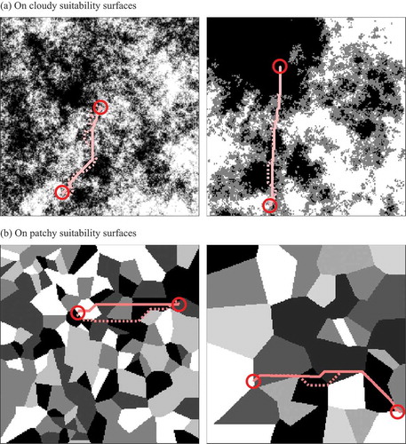
Figure 9. First two pairs of a minisum-unsuitability path (solid line) and maximin-suitability path (dashed line) and maximin-suitability path (dashed line) between two terminal cells (circled) generated (a) on cloudy cost surfaces and (b) on patchy cost surfaces. Note that darker shades represent higher values