
Figures & data
Figure 1. Study area as represented by the source maps (A) Virtual Land Cover Engine (VLCE) and (B) Annual Crop Inventory (ACI). Note that ACI map displays only the 35 ACI classes with validation samples in the accuracy assessment. ACI classes without validation samples were merged into higher level parent classes
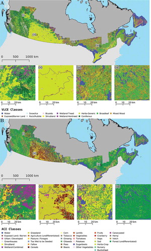
Table 1. Scenarios and approaches used to produce maps in the generalized legend of harmonized land cover classes. The coded name indicates the information used to produce the harmonized map (2 H). Information used comprise E: error matrices, L: Latent Dirichlet Allocation, S: semantic affinity scores, or alternatively ‘~’ when that information was not used. Source maps are VLCE: Virtual Land Cover Engine, and ACI: Annual Crop Inventory
Table 2. Definition of semantic affinity scores between example classes
Table 3. Crosswalk rules from classes in the VLCE legend to classes in the HLC legend
Table 4. Crosswalk rules from classes in the ACI legend to classes in the HLC legend
Figure 2. Reference sample allocation. In the matrix image on the upper left, blanks indicate no such combination and grays indicate no reference sample is allocated. Darker fonts of class names mean higher frequencies. The bar charts on the right of and directly below the image are marginal proportions. Class colors are presented on the right Y-axis and the bottom X-axis of the matrix image. The proportion of reference sample units over areas of agreement and disagreement is presented on the lower-right bar chart
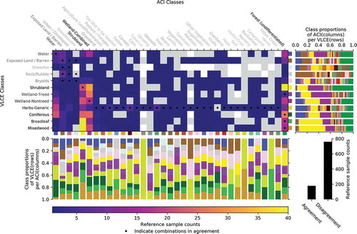
Figure 3. Co-occurrence frequencies (pixel counts) of combinations of source map classes. In the matrix image on the upper left, blanks indicate no such combination. Darker fonts of class names mean higher frequencies. The bar charts on the right of and directly below the image are marginal proportions. Class colors are presented on the right Y-axis and the bottom X-axis of the matrix image. The proportion of combinations in agreement and disagreement is presented on the lower-right bar chart
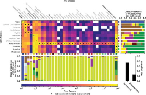
Table 5. Estimates of overall, producer’s (), and user’s (
) accuracy per HLC class over areas of agreement, with standard error. Codes for harmonization scenarios are fully described in
Table 6. Estimates of overall, producer’s (), and user’s (
) accuracy per HLC class over areas of disagreement, with standard error. Codes for harmonization scenarios are fully described in
Figure 4. Harmonized maps by the approaches (A) ‘EL~2H’, using error matrices and LDA outputs for harmonization; and (B) ‘ELS2H’, using error matrices, LDA outputs, and semantic affinity scores for harmonization
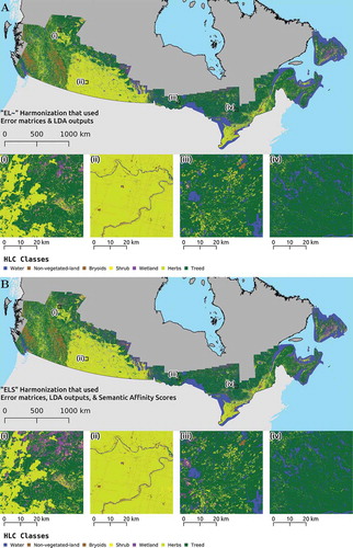
Table 7. For the area of disagreement, the change in accuracy in the harmonized output maps as a function of not using an error matrix, not using an LDA model, and not using semantic affinity scores. Codes for harmonization scenarios are fully described in
Figure 5. Harmonization by the approach ‘EL~2H’, using error matrices and LDA outputs (). HLC labels and their class probabilities of all the combinations of source map classes. Blanks indicate no such combination. Darker fonts of class names mean higher frequencies
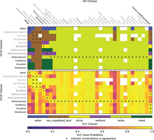
Figure 6. Harmonization by the approach ‘ELS2H’, using error matrices, LDA outputs, and semantic affinity scores (). HLC labels and their class probabilities of all the combinations of source map classes. Blanks indicate no such combination. Darker fonts of class names mean higher frequencies
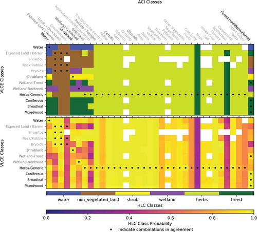
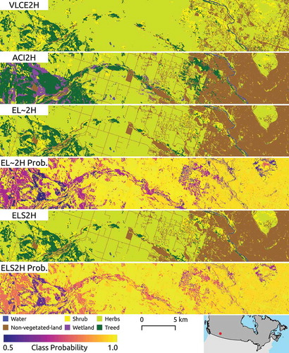
Figure 7. Details of benchmark maps (VLCE2H and ACI2H), harmonized maps (EL~2H and ELS2H), and maps of HLC class probabilities over an example region west of Calgary, Alberta, represented by the red dot in the lower-right map
Data availability statement
The land cover data used in this study are openly available from the National Forest Information System and the Federal Geospatial Platform:
2015 VLCE: https://opendata.nfis.org/downloads/forest_change/CA_forest_VLCE_2015.zip
2015 ACI: https://open.canada.ca/data/en/dataset/ba2645d5-4458-414d-b196-6303ac06c1c9