Exact space–time prism of an activity program: bidirectional searches in multi-state supernetwork

Figures & data

Table 1. Abbreviations used in this study

STP: Space–time prism	AP: Activity program
PPA: Potential path area	ATP: Activity-travel pattern
NTP: Network-time prism	P2P: Point-to-point
TBS: Two-stage bidirectional search	ALT: A*, landmark, and triangular inequalities
SBS: Simultaneous bidirectional search	ALT*: ALT considering fixed activity location(s)

Figure 1. Schematic representation of search spaces. Node $n_i$ $\left(i=1,2,3\right)$ is at the border of a search space. The time expense of pattern H₀ – $n_i$ – H₁ is equal to $t_{\mathrm{B}}-d_a$

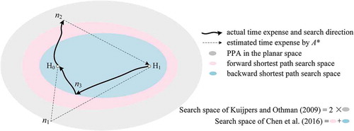
Figure 2. Four-state supernetwork representation of conducting two activities (Liao 2019)

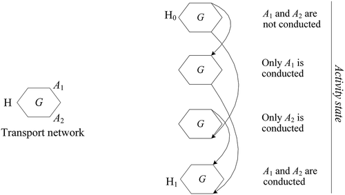
Figure 3. Schematic representation at the search frontier $n{|}_s$ using the method of Liao (2019). The partial ATP from $n{|}_s$ to ${\mathrm{H}}_1$ has activity sequence red→blue→green

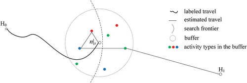
Table 2. Notation list

$G\left(N,E\right)$	Transport network $G$ with $N$ and $E$ being the sets of nodes and links respectively
$n,u,v$	Nodes (locations) in $G$ ($n,u,v\in G$)
$\alpha$, $A$, $S$	An activity, activity set, and activity state set of an AP respectively
$SNK$	Multi-state supernetwork related to the AP
$s$, $s^{\prime }$	Two activity states ($s,s^{\prime }\in S$)
$A_s$	Sub-set of activities that are not conducted at state $s$, $A_s+\overline{A_s}=A$
$\left|\mathrm{\Delta }\right|$	Number of elements of an arbitrary set $\mathrm{\Delta }$ (e.g. $N$, $S$, $A$)
$d_{\alpha }$	Minimum activity duration of $\alpha$ ($\alpha \in A$)
$\left[o_{\alpha u},e_{\alpha u}\right]$	Time window for activity $\alpha$ at $u$
${\mathrm{H}}_0$, ${\mathrm{H}}_1$	Two anchor points in $G$ or $SNK$ (at the first and last activity state respectively)
${ }_0$, $t_1$	Time points at ${\mathrm{H}}_0$ and ${\mathrm{H}}_1$ respectively
$t_{\mathrm{B}}$	Time budget to conduct the AP, $t_{\mathrm{B}}=t_1-t_0$
${|}_s$	Activity state information attached to nodes of $G$
$l\left(\cdot ,\cdot \right)$	Static time expense of a link in $G$ or $SNK$
$t\left(\cdot ,\cdot \right)$	Shortest travel time between any two nodes in $G$, $t\left(\cdot ,\cdot \right)\ge 0$
e(,)	Lower bound of $t\left(\cdot ,\cdot \right)$ by the Euclidean distance and maximum speed
$ALT\left(\cdot ,\cdot \right)$	Lower bound of $t\left(\cdot ,\cdot \right)$ by the ALT method
$g_{v{{|}_s}^{\prime }}\left(n{|}_s\right)$	Actual activity-travel time of a sub-path from $v{|}_{s^{\prime }}$ to $n{|}_s$
$h_{v{|}_{s^{\prime }}}\left(n{|}_s\right)$	Lower bound of $g_{v{|}_{s^{\prime }}}\left(n{|}_s\right)$
$p_{v{|}_{s^{\prime }}}\left(n{|}_s\right)$	Consistent and feasible lower bound of $g_{v{|}_{s^{\prime }}}\left(n{|}_s\right)$
$f_{{\mathrm{H}}_0{\mathrm{H}}_1}(n{|}_s)$	Potential function of a path time expense from ${\mathrm{H}}_0$ to ${\mathrm{H}}_1$ passing $n{|}_s$
$\to ,\leftarrow$	Forward and backward directions respectively placed on the top of notations

Figure 4. Schematic representation of the search space of the naïve SBS method (it is comparable with Figure 1 only when the blue ellipses are drawn on the same scale)

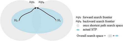
Figure 5. Schematic representation of goal-directed SBS method

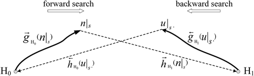
Figure 6. Schematic representation of the search space of the goal-directed SBS method (it is comparable with Figures 1 and 3 only when the blue ellipses are drawn on the same scale)

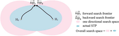
Figure 7. Flowchart of the TBS and SBS methods

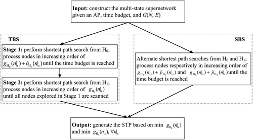
Figure 8. Eindhoven-Helmond corridor (scale: 1:150,000)

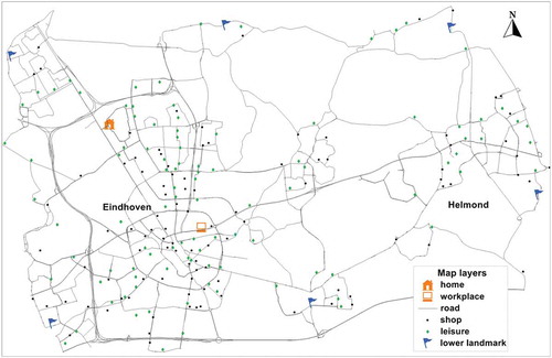
Figure 9. Exact activity state-dependent PPAs (in blue) by car

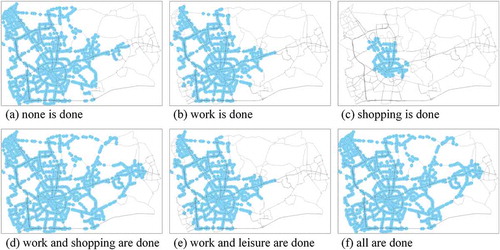
Figure 10. Exact activity state-dependent PPAs (in blue) by bike

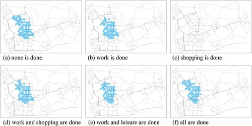
Table 3. Numbers of accessible locations (lower – upper bound in Liao (2019)/exact)

Activity state	Using car		Using bike
	Shop	Leisure	Shop	Leisure
None is done	63–64/77	69–72/77	31–33/25	30–31/26
Work is done	53–59/62	55–61/67	23–29/24	21–26/23
Shopping is done	n/a	11–17/23	n/a	0–0/0
Work and shopping are done	n/a	81–82/87	n/a	26–31/26
Work and leisure are done	56–61/62	n/a	28–33/21	n/a

(n/a: not applicable as the activity is done at the state; the exact numbers of locations are in bold.)

Figure 11. Grid network for one flexible activity

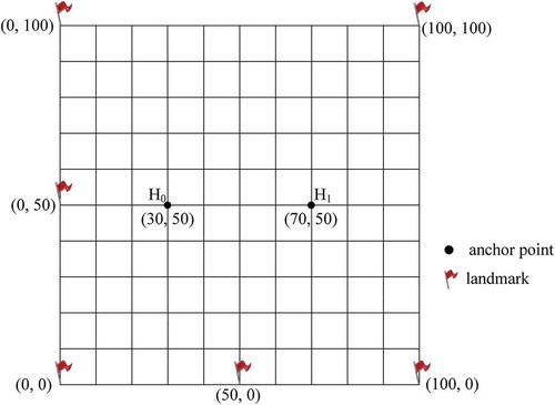
Figure 12. Search spaces of different methods

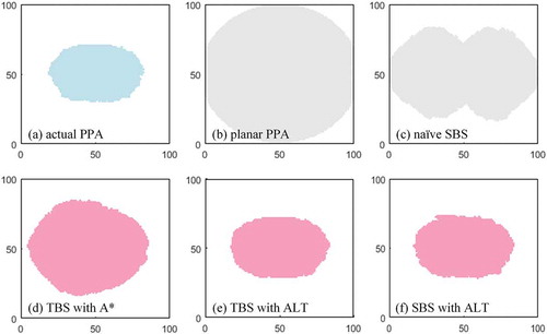
Figure 13. Extra nodes explored beyond the actual PPA of different methods

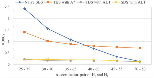
Figure 14. Grid network for one AP of three activities with flexible activity sequences

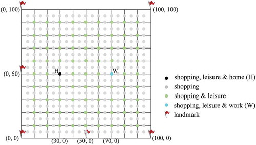
Figure 15. State-dependent PPAs and search spaces of different methods

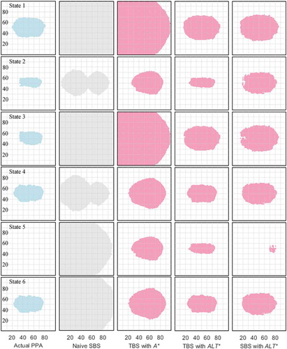
Figure 16. Extra nodes explored beyond the actual PPA of different methods

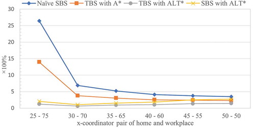
Table 4. Numbers of nodes explored and computation times

	Actual PPA	Naïve SBS	TBS with A*	TBS with ALT*	SBS with ALT*
Number of nodes explored	5,883	46,335	28,111	9,625	12,061
Extra nodes beyond actual PPA	n/a	687%	379%	64%	105%
Computation time (sec)	n/a	0.008	0.007	0.004	0.006

Table 5. Computation time in second for 1000 random pairs (the least times are in bold)

1st AP					2nd AP
Size Method	101^2	251^2	501^2	1001^2	Size Method	101^2	251^2	501^2	1001^2
Naïve SBS	0.481	3.77	20.24	93.32	Naïve SBS	6.48	45.93	219.9	995.4
TBS with A*	0.634	4.88	28.06	117.5	TBS with A*	5.29	32.78	143.7	602.8
TBS with ALT	0.497	3.73	27.49	94.16	TBS with ALT*	3.06	18.41	85.66	355.7
SBS with ALT	0.627	4.69	20.73	114.0	SBS with ALT*	5.34	34.07	173.2	816.2

Liao, F., 2019. Space–time prism bounds of activity programs: A goal-directed search in multi-state supernetworks. International Journal of Geographical Information Science, 33, 900–921.

 Web of Science ®Google Scholar

Data and codes availability statement

The data and codes that support the findings of this study are available in figshare.com with the identifier(s) at the link https://doi.org/10.6084/m9.figshare.13108094.v2.