Geocomplexity explains spatial errors

Figures & data

Figure 1. A measure of spatial local complexity.

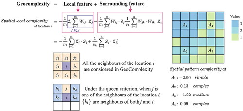
Figure 2. Spatial distributions of Gini coefficients in Australia (a) and major cities, including Brisbane (b), Sydney (c), Perth (d), Adelaide (e) and Melbourne (f).

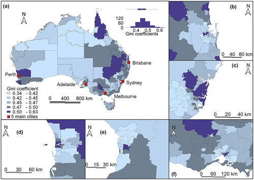
Table 1. A summary of explanatory variables.

Variable name	Unit	Data description	Source
Sex ratio	%	Sex ratio	ABS
Internet coverage	%	Internet accessed from dwelling	ABS
Higher education ratio	%	Higher education level	ABS
Income	AUD	Median income level	ABS
House ownership	%	Percentage of people who owned a house	ABS
Industrial company	count	Number of industrial companies	ABS
Industrial employee	count	Number of industrial employees	ABS
		Industrial land use polygon	OSM
Industrial scale	%	Key industrial infrastructure	OSM
		Key industrial factory	NPI

Figure 3. The workflow for assessing geocomplexity of economic inequality and its contribution to explaining spatial errors.

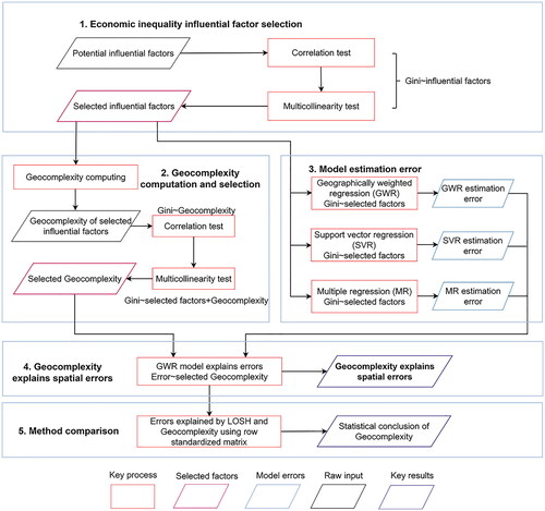
Table 2. Multiple regression for modelling Gini coefficients at the SA3 level.

Variable	Coefficient (significance level)
Intercept	2.65e^–01 (***)
Sex ratio	–9.01e^–03
Income	2.12e^–06 (***)
House ownership	3.04e^–03 (***)
Industrial employee	–2.54e^–06 (***)
Industrial scale	–3.27e^–02
p-value for model	<0.001
R-squared value	0.47
AIC value	–1288

***indicates significance level indicated by a p-value less than 0.001.

Figure 4. The correlation matrix among Gini coefficients selected explanatory variables, and geocomplexities of explanatory variables. Note: ‘x’ indicates that the correlation is not significant.

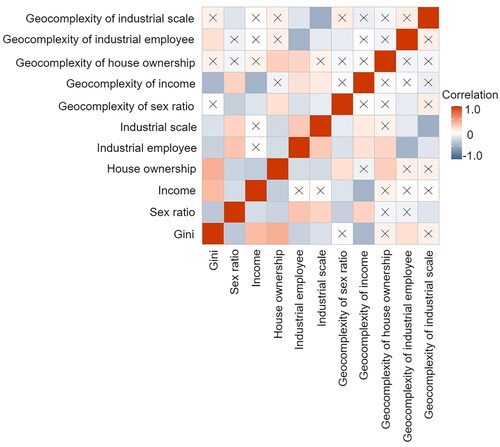
Figure 5. Geocomplexity of selected variables in SA3 regions colored by Gini coefficient. (a) Income level v.s. Geocomplexity of income. (b) Industrial employee counts v.s. Geocomplexity of industrial employees.

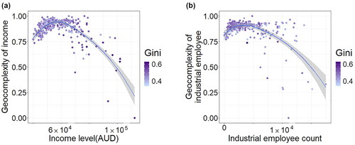
Figure 6. Statistical distribution of model errors. (a) Errors of multiple regression estimations. (b) Errors of SVR estimations. (c) Errors of GWR estimations.

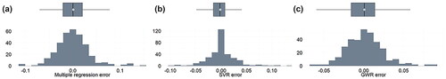
Table 3. Performance of three models.

	MR model	SVR model	GWR model
R^2	0.472	0.646	0.761
RSS (Residual sum of squares)	0.396	0.266	0.179

Figure 7. Residuals of error explanations. (a) Residual-fitted plot of error explanation from three models. (b) Q-Q plot showing residuals of multiple regression error explanation. (c) Q-Q plot showing residuals of SVR error explanation. (d) Q-Q plot showing residuals of GWR error explanation.

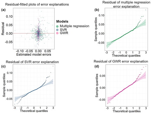
Table 4. A summary of the contribution of geocomplexity in explaining spatial errors.

Count of significant results and explanation model summaries	MR error explanation	SVR error explanation	GWR error explanation
Geocomplexity of income	237	105	53
Geocomplexity of industrial employee	95	70	3
Global ${\mathrm{R}}^2$	0.467	0.166	0.136
AIC value	–1459	–1477	–1575
RSS value	0.211	0.221	0.155

Note: The statistical significance level is 0.05. The total observation count is 333.

Figure 8. Coefficients of geocomplexity of income and industrial employee in multiple regression error explanation. Distribution of geocomplexity of income in Australia (a) and major cities including, Sydney (b) and Melbourne (c). Distribution of geocomplexity of industrial employees in Australia (d) and major cities including, Melbourne (e) and Adelaide (f).

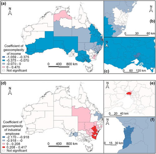
Figure 9. Coefficients of geocomplexity of income and industrial employee in SVR error explanation. Distribution of geocomplexity of income in Australia (a) and major cities including, Brisbane (b) and Melbourne (c). Distribution of geocomplexity of industrial employees in Australia (d) and major cities including, Brisbane (e) and Sydney (f).

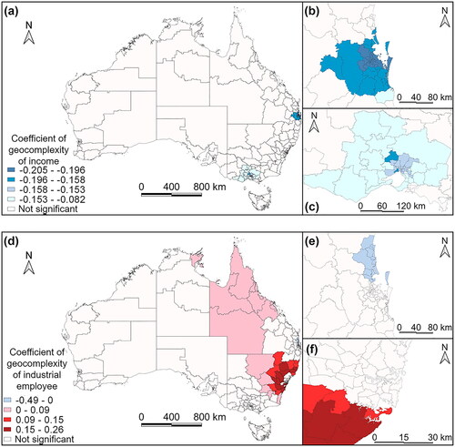
Figure 10. Coefficients of geocomplexity of income and industrial employee in GWR error explanation (a). Distribution of geocomplexity of income in Brisbane (b).

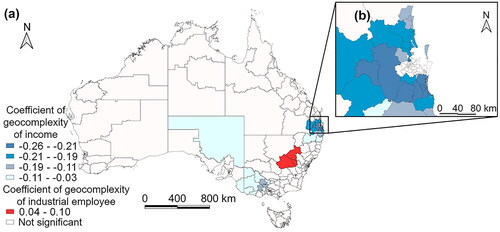
Table 5. The comparison between geocomplexity and local autocorrelation index on error explanation.

Performance (Global $R^2,$ RSS, AIC)	Geocomplexity with binary spatial weight matrix using GWR	Geocomplexity with row standardized spatial weight matrix using GWR	Local autocorrelation index using GWR	Geocomplexity with binary spatial weight matrix using global regression
Multiple regression error explanation model	47%, 0.21, –1459	42%, 0.23, –1430	38%, 0.25, –1418	3%, 0.38, –1299
SVR error explanation model	17%, 0.22, –1477	6%, 0.25, –1444	7%, 0.25, –1448	1%, 0.26, –1426
GWR error explanation model	14%, 0.16, –1575	12%, 0.16, –1567	12%, 0.16, –1569	1%, 0.18, –1556

Bold values show the explanatory power of the optimal geocomplexity indicator for the errors of the three models.

Data and codes availability statement

The data and code that support the findings of this study are available in Figshare at https://doi.org/10.6084/m9.figshare.20500284.v1.