A classification scheme for static origin–destination data visualizations

Figures & data

Figure 1. The OD matrix: (a) An example of an OD data matrix, with regional migration data in 2018, Iceland (Iceland 2023). The numbers represent migrating people. (b) OD data components: connection (true or false); spatial (description of trajectory); time (duration); attribute (qualitative and/or quantitative). (c) OD matrix reading levels (highlighted cells): elementary (cell to cell), intermediate (cell to row or column); overall (all to all). Schematic diagrams on the top show examples of three reading levels. The matrix at the bottom shows the lower right section from the OD matrix in (a).

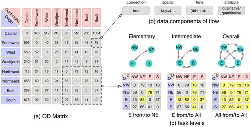
Table 1. The classification scheme and the structure of the section.

Aspects	Variables	Features	Sub-sections
Granularity of flows		Individual flow; grouped flow	4.2
Dimensionality in and of  the display space	Dimensionality of node and flow symbols	0D; 1D; 2D; 3D	4.3.1
	Dimensionality of the display space	2D; 3D	4.3.2
Semantics of the display		Space-related semantics; time-related semantics; attribute-related semantics; hybrid semantics	4.4.1
Representation of nodes  and flows	Representation of nodes	Ungrouped; O/D-grouped; OD-grouped; OD-joint	4.5.1
	Representation of flows	Linking; attaching; intersecting	4.5.2
	Direction of flow symbols	Undirected flow; directed flow	4.5.3
Ways of relating two  visualizations		Relating two visualizations by identifying nodes	4.6.1
		Relating two visualizations by nesting	4.6.2

Figure 2. Appling different semantics to the third dimension, two flows (from A to B, and from A to C) are visualized with example data. (a) Application of space-related semantics to the third dimension. Lines are imitations of plane trajectories. (b) Application of time-related semantics to the third dimension. It is an example of space-time cube. (c) Application of attribute-related semantics to the third dimension, where the third dimension represents the attribute component. (d) Application of attribute-related semantics to the third dimension, where the third dimension represents connection.

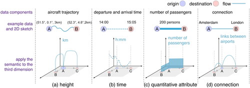
Figure 3. Representation of nodes. The five columns show five categories of node representations. The first row indicates how can the five categories are conceptually transformed. The second row are sketches of four flows between two nodes. The third row shows the context of each category. The last row shows examples of each category.

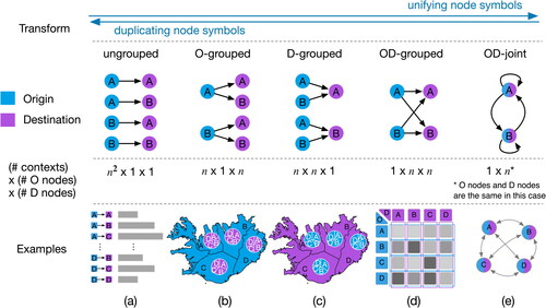
Figure 4. Representation of flows: linking, attaching, and intersecting. In linking, the relation between the origin symbols and the destination symbols is disjoint. In attaching, the relation between the origin symbols and the destination symbols is adjacent or touching. In intersecting, the relation between the origin symbols and the destination symbols is overlap or containment.

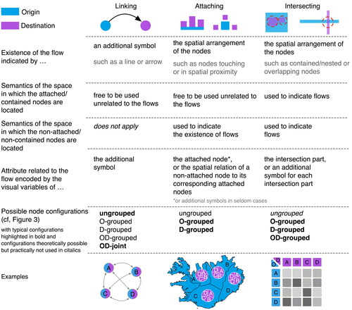
Figure 5. Direction of flow symbols. (a) Undirected flow. (b) Directed flow.

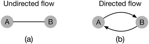
Figure 6. Examples of the identification of nodes. In the two visualizations (Vis-1 and Vis-2), nodes are represented by several node symbols. Node symbols in the two visualizations can be identified in several ways. (a) Positioning: Nodes can be positioned close to each other, in corresponding positions in each visualization, or by other rules. (b) Drawing lines between node symbols, indicating that they are representing the same node. These lines need to differ from flow symbols. (c) Color-coding the node symbols. (d) Brushing: Interaction can be applied to node identification. When selecting the node symbol in Vis-1, the corresponding symbol in Vis-2 will be highlighted. (e) Labelling: Labels are used to identify nodes directly.

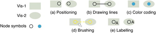
Figure 7. Three possibilities of flow representation when relating two OD visualizations. (a) Flow symbols are connecting origins and destinations within one visualization. (b) Flow symbols are connecting origins and destinations across two different visualizations. (c) Combination of (a) and (b).

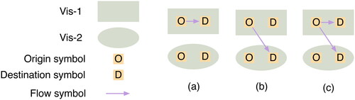
Figure 8. Relating two visualizations by nesting. There are two visualizations (Vis-1 and Vis-2). Multiple Vis-1 are nested into Vis-2, which are positioned where the node symbols in Vis-2 are located.

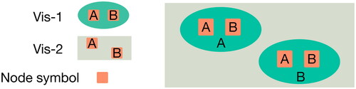
Figure 9. Reordered distance matrix for 54 OD visualization examples. The 54 × 54 matrix represents distances among 54 OD visualizations. It is reordered by the single-linkage clustering method. Certain visualizations are more similar than others, and these are grouped in a blue rectangle.

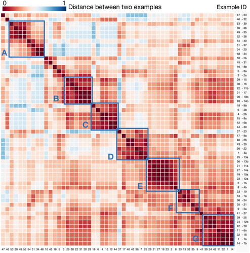
Table 2. Classifying existing OD visualization examples in the literature.

	Aspects	Granularity of flows		Dimensionality in and of the display space										Semantic of the display space				Representation of nodes and flows									Relating two visualizations
	Variables			Node symbols				Flow symbols				Display space						Nodes				Flows			Direction of flows
ID	Example OD visualization	Features
		Individual	Grouped	0D	1D	2D	3D	0D	1D	2D	3D	2D	3D	Space- related	Time- related	Attribute- related	Hybrid	Ungrouped	O/D- grouped	OD- grouped	OD- joint	Linking	Attaching	Intersecting	Undirected	Directed	Identification of nodes	Nesting
1a	Necklace map (Speckmann and Verbeek 2010) using a ‘necklace’ to show flows between regions		■			■				■		■					■				■	■				■	■
1b	Necklace map; using a Choropleth map to show nodes		■			■						■		■							■
2a	Brushing between pie chart and OD matrix: pie chart		■			■				■		■				■			■				■		■		■
2b	Brushing between pie chart and OD matrix: OD matrix		■		■					■		■				■				■				■		■
3a	Cluster heat map (Wilkinson et al. 1994): Tree		■	■						■		■				■			■			■			■		■
3b	Cluster heat map: Matrix		■		■			■				■				■				■				■	■
4a	Grouse (Archambault et al. 2007); use graph to visualize flows	■				■			■			■				■					■	■			■		■
4b	Grouse; ‘Metanodes’ showing hierarchy in the graph		■			■						■				■					■
5a	Flowstrate (Boyandin 2013): Two maps showing origins and destinations		■			■			■			■		■						■		■				■	■
5b	Flowstrate: heatmap showing temporal flows		■	■				■				■					■	■					■			■
6a	Maptrix (Yang et al. 2017): two maps showing origins and destinations		■			■				■		■					■			■		■				■	■
6b	Maptrix: OD matrix		■		■			■				■				■				■				■		■
7a	Multivariate network visualization (van den Elzen and van Wijk 2014): Low-level detail view	■		■					■			■		■							■	■				■	■
7b	Multivariate network exploration: High-level overview		■			■				■		■					■				■	■				■
8a	TimeMatrix (Yi et al. 2010). Matrix layout		■		■					■		■				■				■				■		■		■
8b	TimeMatrix: ‘TimeCell’ showing temproal flows		■	■						■		■					■	■					■		■
9a	NodeTrix (Henry et al. 2007): node-link diagram		■			■			■			■				■					■	■			■			■
9b	NodeTrix: matrix embedded into the nodes of node-link diagram	■			■			■				■				■				■				■		■
10a	Pie chart map: map representing origins and destinations					■						■		■							■							■
10b	Pie chart map: pie chart embedded into map regions		■			■				■		■				■			■				■			■
11a	Map^2 (Guo et al. 2006): the overall matrix which is a schematic ‘map’			■		■						■		■							■							■
11b	Map^2: small maps showing flows moved from other states into a specific state		■			■				■		■		■					■				■			■
12a	Interchange Circos diagram map (Zeng et al. 2013): the map showing flows between regions					■						■		■							■							■
12b	Interchange Circos diagram map: the Circos diagram which shows interchange among nodes		■			■				■		■				■					■	■				■
13a	Shifted Maps (Otten et al. 2018):Node-link diagram representing topologies of movement	■				■				■		■				■					■	■			■			■
13b	Shifted Maps: Maps showing location											■		■							■
14a	Map with flow diagrams (Andrienko et al. 2017a): map representing origins and destinations					■						■		■							■							■
14b	Map with flow diagrams: flow diagram showing incoming/outgoing flows		■			■				■		■				■			■				■			■
15	Treemaps (Shneiderman 1992)		■			■				■		■				■			■					■		■		■
16	OD maps (Wood et al. 2010)		■			■				■		■		■					■					■		■		■
17	Stacked bar chart (Streit and Gehlenborg 2014)		■			■				■		■				■			■				■			■	–	–
18	Automated layout flow map (Stephen 2016)		■			■				■		■					■				■	■				■
19	Minard’s flow map (Minard 1869)	■		■						■		■					■				■	■				■
20	The space–time cube (Kraak 2008)	■			■						■		■				■				■	■				■
21	Node-link diagrams with animated edge texture (Romat et al. 2018)		■	■					■			■		■							■	■				■
22	Node-link diagram (Battista et al. 1994)	■		■					■			■				■					■	■			■
23	3D node-link diagram (Munzner 1997)	■		■					■				■			■					■	■			■
24	City flow (Nagel et al. 2017)	■		■						■		■		■							■	■				■
25	Sankey diagram (Sankey 1898, Schmidt 2008)		■	■						■		■				■					■	■				■
26	Arc diagram (Wattenberg 2002)	■			■					■		■				■					■	■			■
27	Alluvial diagram (Holtz 2018)		■		■					■		■					■			■		■				■
28	Circos (Krzywinski et al. 2009)		■			■				■		■				■					■	■				■
29	Hive plots (Krzywinski et al. 2012)	■			■					■		■				■					■	■			■
30	OD heat map (Loua 1873)		■		■			■				■				■				■				■		■
31	Timeline (Rosenberg and Grafton 2013)	■		■				■				■					■	■					■			■
32	The 3D OD matrix		■		■	■			■				■			■				■				■		■
33	The 3D prism map (Franklin and Lewis 1978)		■				■				■		■				■		■				■			■
34	Stacking-based trajectory visualization (Tominski et al. 2012)	■			■						■		■				■				■	■				■
35	3D display of internet traffic (Cox and Eick 1995)		■	■							■		■				■				■	■			■
36	VisLink (Collins and Carpendale 2007)		■	■							■		■				■		■			■			■
37	3D trajectory visualization (Buschmann et al. 2016)	■		■							■		■	■							■	■				■
38	3D network on a globe (Cox et al. 1996)		■	■							■		■				■				■	■			■
39	3D Network in geographic environment (Hu et al. 2013)		■	■							■			■			■				■	■			■
40	Network in VR globe (Zhang et al. 2018)		■	■							■		■	■							■	■				■

Figure 10. Reordered distance matrix showing the correlation among the 25 features.

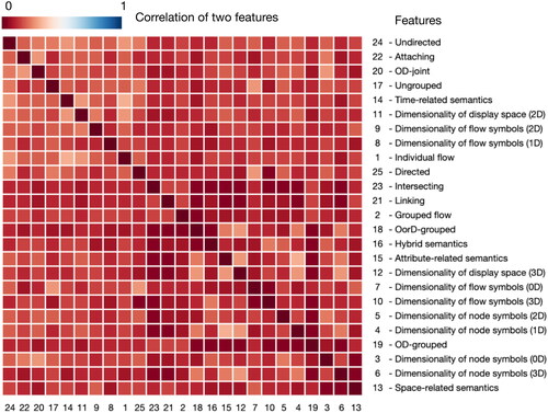
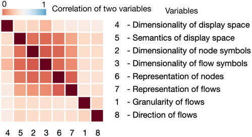
Figure 11. Reordered distance matrix showing the correlation of the eight variables.

Iceland, S., ed. 2023. Internal migration between regions by sex and age 1986–2018. Available from: https://px.hagstofa.is/pxen/pxweb/en/Ibuar/Ibuar__buferlaflutningar__buferlaflinnanlands__buferlaflinnanlandseldra/MAN01001.px/table/tableViewLayout1/?rxid=79b1787a-a295-4882-98ba-2190fb8d1889.

 Google Scholar

Speckmann, A. and Verbeek, K., 2010. Necklace maps. IEEE Transactions on Visualization and Computer Graphics, 16 (6), 881–889.

 PubMed Web of Science ®Google Scholar

Wilkinson, L., et al., 1994. SYSTAT for DOS: advanced applications, version 6 edition. Evanston, IL: SYSTAT Inc.

 Google Scholar

Archambault, D., Munzner, T., and Auber, D., 2007. Grouse: feature-based, steerable graph hierarchy exploration.

 Google Scholar

Boyandin, I., 2013. Visualization of temporal origin-destination data.

 Google Scholar

Yang, Y., et al., 2017. Many-to-many geographically-embedded flow visualisation: an evaluation. IEEE Transactions on Visualization and Computer Graphics, 23 (1), 411–420.

 PubMed Web of Science ®Google Scholar

van den Elzen, S. and van Wijk, J.J., 2014. Multivariate network exploration and presentation: from detail to overview via selections and aggregations. IEEE Transactions on Visualization and Computer Graphics, 20 (12), 2310–2319.

 PubMed Web of Science ®Google Scholar

Yi, J.S., Elmqvist, N., and Lee, S., 2010. Timematrix: analyzing temporal social networks using interactive matrix-based visualizations. International Journal of Human–Computer Interaction, 26 (11–12), 1031–1051.

 Web of Science ®Google Scholar

Henry, N., Fekete, J.D., and McGuffin, M.J., 2007. NodeTrix: a hybrid visualization of social networks. IEEE Transactions on Visualization and Computer Graphics, 13 (6), 1302–1309.

 PubMed Web of Science ®Google Scholar

Guo, D., et al., 2006. A visualization system for space-time and multivariate patterns (VIS-STAMP). IEEE Transactions on Visualization and Computer Graphics, 12 (6), 1461–1474.

 PubMed Web of Science ®Google Scholar

Zeng, W., et al., 2013. Visualizing interchange patterns in massive movement data. Computer Graphics Forum, 32 (3pt3), 271–280.

 Google Scholar

Otten, H., et al., 2018. Shifted maps: revealing spatio-temporal topologies in movement data. In: Proceedings of the IEEE VIS arts program, VISAP 2018.

 Google Scholar

Andrienko, G., et al., 2017a. Revealing patterns and trends of mass mobility through spatial and temporal abstraction of origin-destination movement data. IEEE Transactions on Visualization and Computer Graphics, 23 (9), 2120–2136.

 PubMed Web of Science ®Google Scholar

Shneiderman, B., 1992. Tree visualization with tree-maps: 2-D space-filling approach. ACM Transactions on Graphics, 11 (1), 92–99.

 Web of Science ®Google Scholar

Wood, J., Dykes, J., and Slingsby, A., 2010. Visualisation of origins, destinations and flows with OD maps. The Cartographic Journal, 47 (2), 117–129.

 Web of Science ®Google Scholar

Streit, M. and Gehlenborg, N., 2014. Points of view: bar charts and box plots. Nature Methods, 11 (2), 117.

 PubMed Web of Science ®Google Scholar

Stephen, D.M., 2016. Automated layout of origin-destination flow maps: US county-to-county migration 2009–2013.

 Google Scholar

Minard, C.J., 1869. Carte figurative des pertes successives en hommes de l’Armée Française dans la campagne de Russie 1812–1813. Paris, France: Graphics Press.

 Google Scholar

Kraak, M.-J., 2008. Geovisualization and time – new opportunities for the space-time cube. In: Geographic visualization: concepts, tools and applications. West Sussex, England: John Wiley & Sons, Ltd., 293–306.

 Google Scholar

Romat, H., et al., 2018. Animated edge textures in node-link diagrams: a design space and initial evaluation.

 Google Scholar

Battista, G.D., et al., 1994. Algorithms for drawing graphs: an annotated bibliography. Computational Geometry, 4 (5), 235–282.

 Web of Science ®Google Scholar

Munzner, T., 1997. H3: laying out large directed graphs in 3D hyperbolic space. In: Proceedings of the IEEE symposium on information visualization, 2–10. Available from: https://www.scopus.com/inward/record.uri?eid=2-s2.0-0031353494&partnerID=40&md5=02cf763b0e27d296f17cd4396335389c.

 Google Scholar

Nagel, T., Pietsch, C., and Dork, M., 2017. Staged analysis: from evocative to comparative visualizations of urban mobility. In: 2017 IEEE VIS arts program (VISAP), 1–8.

 Google Scholar

Sankey, H.R., 1898. Introductory note on the thermal efficiency of steam‐engines.. In: Minutes of proceedings of the institution of civil engineers, vol. 134, 278–283.

 Google Scholar

Schmidt, M., 2008. The Sankey diagram in energy and material flow management. Journal of Industrial Ecology, 12 (1), 82–94.

 Web of Science ®Google Scholar

Wattenberg, M., 2002. Arc diagrams: visualizing structure in strings. In: Proceedings – IEEE symposium on information visualization, INFO VIS, 110–116.

 Google Scholar

Holtz, Y., 2018. Researcher network and migration flows. Available from: https://www.data-to-viz.com/story/AdjacencyMatrix.html.

 Google Scholar

Krzywinski, M., et al., 2009. Circos: an information aesthetic for comparative genomics. Genome Research, 19 (9), 1639–1645.

 PubMed Web of Science ®Google Scholar

Krzywinski, M., et al., 2012. Hive plots – rational approach to visualizing networks. Briefings in Bioinformatics, 13 (5), 627–644.

 PubMed Web of Science ®Google Scholar

Loua, T., 1873. Atlas Statistique de la Population de Paris. Paris: J. Dejey and Co. Editeurs.

 Google Scholar

Rosenberg, D. and Grafton, A., 2013. Cartographies of time: A history of the timeline. New York: Princeton Architectural Press.

 Google Scholar

Franklin, R., and Lewis, H.R., 1978. 3-D graphic display of discrete spatial data by prism maps. In: Proceedings of the 5th annual conference on Computer graphics and interactive techniques, 70–75.

 Google Scholar

Tominski, C., et al., 2012. Stacking-based visualization of trajectory attribute data. IEEE Transactions on Visualization and Computer Graphics, 18 (12), 2565–2574.

 PubMed Web of Science ®Google Scholar

Cox, K.C. and Eick, S.G., 1995. Case study: 3D displays of internet traffic. In: Information visualization, 1995. Proceedings. IEEE, 129–131.

 Google Scholar

Collins, C. and Carpendale, S., 2007. VisLink: revealing relationships amongst visualizations. IEEE Transactions on Visualization and Computer Graphics, 13 (6), 1192–1199.

 PubMed Web of Science ®Google Scholar

Buschmann, S., Trapp, M., and Döllner, J., 2016. Animated visualization of spatial–temporal trajectory data for air-traffic analysis. The Visual Computer, 32 (3), 371–381.

 Web of Science ®Google Scholar

Cox, K.C., Eick, S.G., and He, T., 1996. 3D geographic network displays. SIGMOD Record (ACM Special Interest Group on Management of Data), 25 (4), 50–54. Available from: https://www.scopus.com/inward/record.uri?eid=2-s2.0-0002766331&partnerID=40&md5=878279d380753ae5f0ccd6a8ad00172c.

 Google Scholar

Hu, H., Zhang, H., and Li, W., 2013. Visualizing network communication in geographic environment. In: Proceedings – 2013 international conference on virtual reality and visualization, ICVRV 2013, 206–212.

 Google Scholar

Zhang, M.-J., et al., 2018. Visual exploration of 3D geospatial networks in a virtual reality environment. The Computer Journal, 61 (3), 447–458.

 Web of Science ®Google Scholar

Data and codes availability statement

The data and codes are available on figshare.com with the link: https://doi.org/10.6084/m9.figshare.21176320.v3. The data is a matrix created according to Table 2 in this manuscript. The code computes the three functions in Section 5 correspondingly.