Figures & data
Figure 1 The first eight Walsh functions.
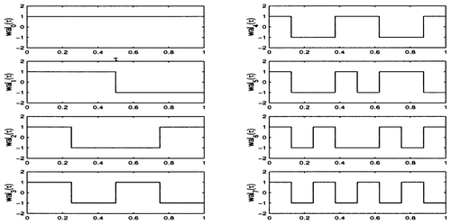
Figure 2 Approximation of f(τ) = sin(2πτ) in S 3.
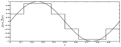
Figure 3 Inverse Laplace transform g(t) of and its stairstep approximation [gbar](t) in S
5.
 in S 5.](/cms/asset/7f817c71-53a4-4e2f-99c6-a79650315ffb/nmcm_a_106689_o_f0003g.gif)
Figure 4 Inverse Laplace transform J
0(t) of and its stairstep approximation [Jbar]
0(t) in S
5.
![Figure 4 Inverse Laplace transform J 0(t) of and its stairstep approximation [Jbar] 0(t) in S 5.](/cms/asset/45b44893-decf-463a-bf4c-ddb650fccda6/nmcm_a_106689_o_f0004g.gif)
Figure 5 Solutions x(t,zi
) of the heat
Equationequation (29) according to Equation(31)
and its stairstep approximations [xbar](t, zi
) in S
5 for z
1 = 0.2,z
2 = 0.4,z
3 = 0.6,z
4 = 0.8.
 in S 5 for z 1 = 0.2,z 2 = 0.4,z 3 = 0.6,z 4 = 0.8.](/cms/asset/9baa8236-27e5-47fd-a4cb-6875a37b6f56/nmcm_a_106689_o_f0005g.gif)
Figure 6 Time-variable PI controller.
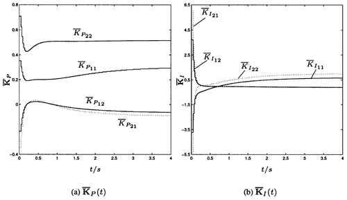
Figure 7 Closed-loop step response of the time-variant plant with [Kbar]
P
(t) and [Kbar]
I
(t) from
in comparison with the desired decoupled closed-loop behaviour according to Equation(35) for w
1(t) = σ(t − 0.6), w
2(t) = 0.
![Figure 7 Closed-loop step response of the time-variant plant with [Kbar] P (t) and [Kbar] I (t) from figure 6 in comparison with the desired decoupled closed-loop behaviour according to Equation(35) for w 1(t) = σ(t − 0.6), w 2(t) = 0.](/cms/asset/b3dff2d3-5730-4310-94d8-51540d14d162/nmcm_a_106689_o_f0007g.gif)
Figure 8 Closed-loop step response of the time-variant plant with [Kbar]
P
(t) and [Kbar]
I
(t) from
in comparison with the desired decoupled closed-loop behaviour according to Equation(35) for w
1(t) = 0, w
2(t) = σ(t − 0.6).
![Figure 8 Closed-loop step response of the time-variant plant with [Kbar] P (t) and [Kbar] I (t) from figure 6 in comparison with the desired decoupled closed-loop behaviour according to Equation(35) for w 1(t) = 0, w 2(t) = σ(t − 0.6).](/cms/asset/8684ad25-5648-478d-937d-54b478941368/nmcm_a_106689_o_f0008g.gif)