Figures & data
Figure 1. (a) Marker clusters generally moving with respect to global coordinate system O
G
(x
G
, y
G, z
G
) are used to define local coordinate systems (LCS) fixed in the femur O
F
(x
F
, y
F, z
F
) and in the tibia O
T
(x
T
, y
T, z
T
), respectively. In the present model the FE and the TR axes intersect at point I but need not to be orthogonal. Angle describes the FE-movement whereas
describes the tibial rotation. (b) Two additional LCS are defined. The first is fixed in the femur (x
1, y
1, z
1), and the second is fixed in the tibia (x
2, y
2, z
2). The origins of the two LCS coincide with the point I. The
axis lies in the FE axis whereas
coincides with the TR axis. The angle
represents the angle between FE and TR axes.
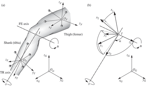
Figure 2. (a) Passive knee flexion with and without external load. Solid line [Citation30]: constraint based model; short dashed line [Citation30]: reference model; dash-dotted line [Citation31]: external torque of 3 Nm; dotted line [Citation31]: internal torque of 3 Nm; long dashed line [Citation32]; (b) FE angle and TR angle during a gait cycle [Citation33]. Note that (b) shows and
whereas (a) plots
. In addition, the range of
is about 90° in (a) and 35° in (b).
![Figure 2. (a) Passive knee flexion with and without external load. Solid line [Citation30]: constraint based model; short dashed line [Citation30]: reference model; dash-dotted line [Citation31]: external torque of 3 Nm; dotted line [Citation31]: internal torque of 3 Nm; long dashed line [Citation32]; (b) FE angle and TR angle during a gait cycle [Citation33]. Note that (b) shows and whereas (a) plots . In addition, the range of is about 90° in (a) and 35° in (b).](/cms/asset/3dd863bf-91a9-4ba2-b6ad-1ca5250f6a65/nmcm_a_507094_o_f0002g.gif)
Figure 3. Rescaled values of the residual near the true solution (problem with exact data).
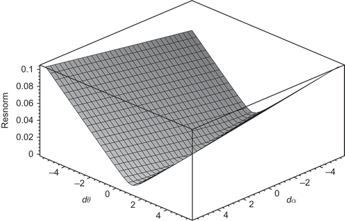
Figure 4. Differences between the optimized parameters and the true simulation input values for model two with the orthogonality constraint and function fitted to data from [Citation19] (a) and [Citation32] (b).
![Figure 4. Differences between the optimized parameters and the true simulation input values for model two with the orthogonality constraint and function fitted to data from [Citation19] (a) and [Citation32] (b).](/cms/asset/9714add8-c7a5-49e1-a299-07bfe18a402f/nmcm_a_507094_o_f0004g.gif)
Figure 5. Residual rotation angles for model two with the orthogonality constraint and fitted to data from [Citation19] (a) and [Citation32] (b).
![Figure 5. Residual rotation angles for model two with the orthogonality constraint and fitted to data from [Citation19] (a) and [Citation32] (b).](/cms/asset/972217a1-3992-4996-a65e-8b65158a5572/nmcm_a_507094_o_f0005g.gif)
Figure 6. Noisy data: square root of the mean squared difference for the model parameters in the model without (left) and with (right) orthogonality constraint. The standard deviation of the input parameters is
(solid lines) and
(dashed lines);
: circle;
: triangle;
: cross;
: X. Function
is fitted to data from [Citation19] (a) and [Citation32] (b).
![Figure 6. Noisy data: square root of the mean squared difference for the model parameters in the model without (left) and with (right) orthogonality constraint. The standard deviation of the input parameters is (solid lines) and (dashed lines); : circle; : triangle; : cross; : X. Function is fitted to data from [Citation19] (a) and [Citation32] (b).](/cms/asset/e8fb1f62-3456-4704-8812-5569fe5b1962/nmcm_a_507094_o_f0006g.gif)
Figure 7. Mean residual rotation angles for the model with and without orthogonality constraint. The standard deviation of the input parameters was (solid lines) and
(dashed lines). Function
is fitted to data from [Citation19] (a) and [Citation32] (b).
![Figure 7. Mean residual rotation angles for the model with and without orthogonality constraint. The standard deviation of the input parameters was (solid lines) and (dashed lines). Function is fitted to data from [Citation19] (a) and [Citation32] (b).](/cms/asset/2bc3f0c6-bff6-41f6-9f8c-e9ec4ffab86e/nmcm_a_507094_o_f0007g.gif)