Parameter preserving model order reduction for MEMS applications

Figures & data

Figure 1. 2D model of anemometer. Left: schematics. Right: calculated temperature profile for anemometer function.

Figure 2. Finite element model of the gyroscope.

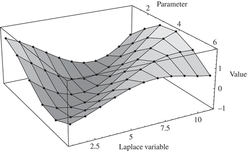
Figure 3. Solution of the transfer function.

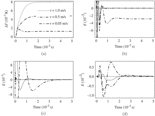
Figure 4. Transient response of anemometer for different velocities (v = 1 m/s, v = 0.5 m/s, v = 0.05 m/s) and relative error of reduced models. (a) Response signal. (b) Relative error for the explicit moment matching model. (c) Relative error for the model reduced with explicit moment matching with averaging. (d) Relative error for the implicit moment-matching model.

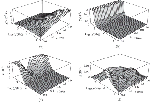
Figure 5. Harmonic analysis of anemometer for different velocities and relative error of reduced models. (a) Response signal. (b) Relative error for explicit moment-matching model. (c) Relative error for the model reduced with explicit moment matching with averaging. (d) Relative error for the implicit moment matching.

Figure 6. Steady-state response of completely parameterized anemometer model (left) and relative error of reduced model (right).

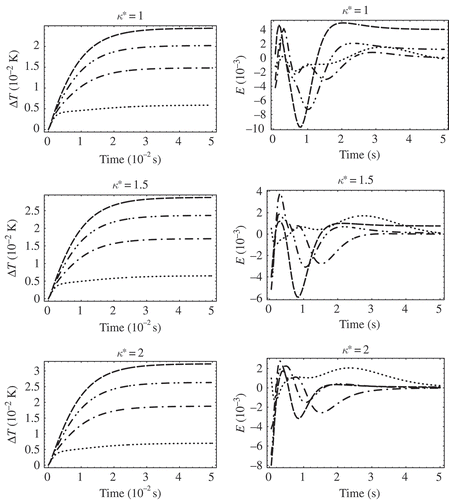
Figure 7. Transient response of the completely parameterized anemometer model (left) and relative error of reduced model (right). Fluid speeds are varied inside one graph with values 0.1 m/s, 0.7 m/s, 1.4 m/s and 2 m/s, thermal conductivity varies between graphs as indicated.

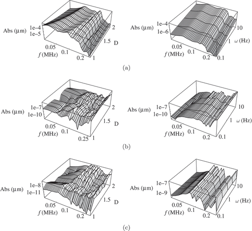
Figure 8. Harmonic analysis of gyroscope depending on the beam thickness (D) and the rotation velocity . (a) Response of original model. (b) Absolute error of reduced model with reduction along all parameters. (c) Absolute error of reduced model with interpolation approach.

Table 1. Computational cost of reduction and simulation for the simplified anemometer model

	Reduction(s)	Stationary(s)	Transient(s)	Harmonic(s)
Original model	–	30.6	26.3	266.0
Explicit method	5.2	0.38	0.49	3.6
Mod. explicit method	13.2	0.43	0.54	3.9
Implicit method	25.3 + 25.4	0.39	0.52	3.7

Table 2. Computational cost of reduction and simulation for the anemometer model including all parameters

	Reduction(s)	Stationary(s)	Transient(s)
Original model	–	82.0	59.5
Reduced model	222.2 + 122.8	4.1	2.4

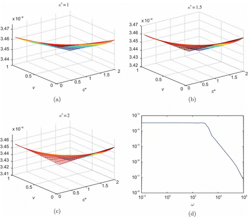
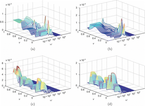
Figure 9. Absolute errors of reduced anemometer model for different interpolation methods and varying error tolerance. (a) BT/rational interpolation with use of error tolerance . (b) BT/rational interpolation with use of error tolerance . (c) BT/polynomial interpolation with use of error tolerance . (d) BT/polynomial interpolation with use of error tolerance .

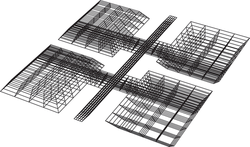
Figure 10. Errors of the completely parameterized anemometer model reduced for different values of the thermal conductivity . (a) Approximated error for . (b) Approximated error for . (c) Approximated error for . (d) Absolute error over frequency domain for .