1,093
Views
33
CrossRef citations to date
0
Altmetric
Original Articles

Interaction of robot swarms using the honeybee-inspired control algorithm BEECLUST

, , , &
Pages 87-100 | Received 29 Apr 2011, Accepted 11 May 2011, Published online: 01 Aug 2011

Figures & data

Figure 1. Aggregation behaviour of young honeybees. The ambient temperature in the arena is 30 °C. On the left side is a temperature optimum with 36 °C (marked with a black line in (b) and (c)). (a) Trajectory of a single bee. The single bee does not show a clear preference to the temperature optimum. (b) A group of bees are released in the centre of the arena (t = 0 min). (c) At the end of the experiment, most of the bees are clustered in the temperature optimum (t = 30 min).
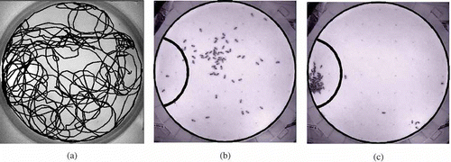
Figure 1. Aggregation behaviour of young honeybees. The ambient temperature in the arena is 30 °C. On the left side is a temperature optimum with 36 °C (marked with a black line in (b) and (c)). (a) Trajectory of a single bee. The single bee does not show a clear preference to the temperature optimum. (b) A group of bees are released in the centre of the arena (t = 0 min). (c) At the end of the experiment, most of the bees are clustered in the temperature optimum (t = 30 min).

Figure 2. Finite-state machine of the BEECLUST controller. Boxes represent the different behavioural states of a robot. Asterisk indicates the starting state of the algorithm. Diamonds represent control structures (if–else decisions).
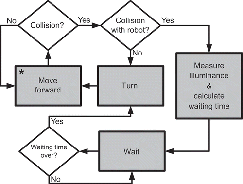
Figure 2. Finite-state machine of the BEECLUST controller. Boxes represent the different behavioural states of a robot. Asterisk indicates the starting state of the algorithm. Diamonds represent control structures (if–else decisions).

Figure 3. (a) A single Jasmine III robot. (b) A swarm of Jasmine III robots in a real-life experiment. Most of the robots are aggregated in the bright area of the arena. Reprinted from [Citation15].

Figure 3. (a) A single Jasmine III robot. (b) A swarm of Jasmine III robots in a real-life experiment. Most of the robots are aggregated in the bright area of the arena. Reprinted from [Citation15].

Figure 4. Screenshot of two robot swarms acting in the simulation environment SMARS. The white spot is the optimum for the ‘light finders’ with 1000 lux and the black spot is the optimum for the ‘shadow finders’ with 0 lux. The ambient illuminance is 500 lux. Robots are represented by boxes which indicate their caste: dark boxes are ‘light finders’ and bright boxes are ‘shadow finders’. The line shows a trajectory of a randomly chosen robot for demonstration purposes. Note: SMARS, Small Robot Simulator.

Figure 4. Screenshot of two robot swarms acting in the simulation environment SMARS. The white spot is the optimum for the ‘light finders’ with 1000 lux and the black spot is the optimum for the ‘shadow finders’ with 0 lux. The ambient illuminance is 500 lux. Robots are represented by boxes which indicate their caste: dark boxes are ‘light finders’ and bright boxes are ‘shadow finders’. The line shows a trajectory of a randomly chosen robot for demonstration purposes. Note: SMARS, Small Robot Simulator.

Figure 5. (a) Overhead screenshot of the arena in SMARS. The bright area indicates the light spot and the dark area indicates the shadow spot. Arena length = 49 patches, arena width = 29 patches. (b) Sensor values detected by the robots. Samples are taken from patches with y = 0, which is the vertical centre of the arena.
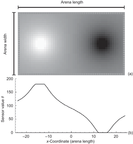
Figure 5. (a) Overhead screenshot of the arena in SMARS. The bright area indicates the light spot and the dark area indicates the shadow spot. Arena length = 49 patches, arena width = 29 patches. (b) Sensor values detected by the robots. Samples are taken from patches with y = 0, which is the vertical centre of the arena.

Table 1. Constants and their values used in Equation1–3 in our simulation runs

Figure 6. Illustration of the dependence between the local illuminance and the waiting time . The solid drawn function was implemented in the ‘light finders’, and the dashed drawn function was implemented in the ‘shadow finders’.
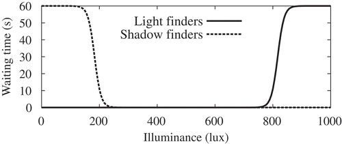
Figure 6. Illustration of the dependence between the local illuminance and the waiting time . The solid drawn function was implemented in the ‘light finders’, and the dashed drawn function was implemented in the ‘shadow finders’.

Figure 7. Fraction of aggregated ‘light finders’ AL (NL ) in target zone over the last minute of observation. The optimal swarm population for the given environment was found at 9 robots. The tested swarm populations were 2, 3, 6, 9, 12, 18, 24, 33, 42, 60, 100 and 120 individuals; n = 6 repetitions per experiment.
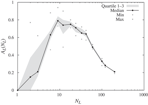
Figure 7. Fraction of aggregated ‘light finders’ AL (NL ) in target zone over the last minute of observation. The optimal swarm population for the given environment was found at 9 robots. The tested swarm populations were 2, 3, 6, 9, 12, 18, 24, 33, 42, 60, 100 and 120 individuals; n = 6 repetitions per experiment.

Figure 8. Fractions of ‘light finders’ aggregated in the target zone within the last minute of observation (median ± quartiles, min and max). is the total number of ‘light finders’ and n = 6 repetitions per experiment.
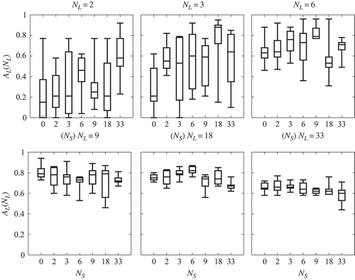
Figure 8. Fractions of ‘light finders’ aggregated in the target zone within the last minute of observation (median ± quartiles, min and max). is the total number of ‘light finders’ and n = 6 repetitions per experiment.

Figure 9. Time in which 50% of the ‘light finder’ swarm aggregated in the target zone () at different population sizes of ‘shadow finders’ (median quartiles, min and max). is the number of ‘light finders’ and n = 6 repetitions per experiment.
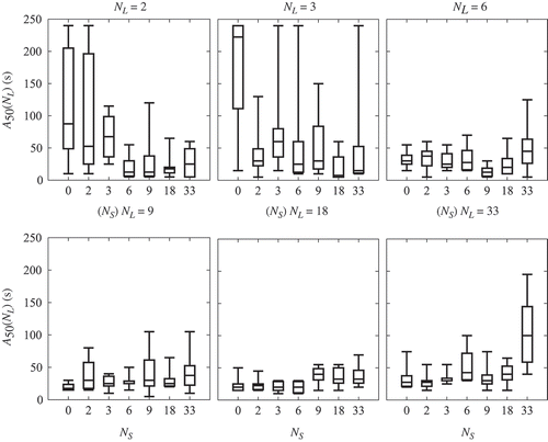
Figure 9. Time in which 50% of the ‘light finder’ swarm aggregated in the target zone () at different population sizes of ‘shadow finders’ (median quartiles, min and max). is the number of ‘light finders’ and n = 6 repetitions per experiment.

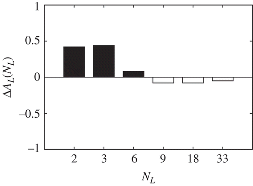
Figure 10. The enhancement of aggregation which is the difference of fraction between and , for , is shown. For details on the formulation of , see EquationEquation (10).

Figure 10. The enhancement of aggregation which is the difference of fraction between and , for –, is shown. For details on the formulation of , see EquationEquation (10)(10).

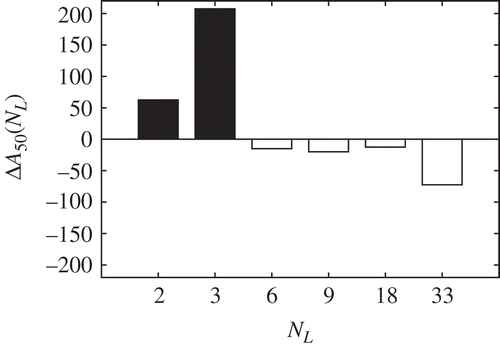
Figure 11. The acceleration of aggregation in seconds which is the difference of between and , for , is shown. For details on the formulation of , see EquationEquation (11).

Figure 11. The acceleration of aggregation in seconds which is the difference of between and , for –, is shown. For details on the formulation of , see EquationEquation (11)(11).

Reprints and Corporate Permissions

Please note: Selecting permissions does not provide access to the full text of the article, please see our help page How do I view content?

To request a reprint or corporate permissions for this article, please click on the relevant link below:

Academic Permissions

Please note: Selecting permissions does not provide access to the full text of the article, please see our help page How do I view content?

Obtain permissions instantly via Rightslink by clicking on the button below:

If you are unable to obtain permissions via Rightslink, please complete and submit this Permissions form. For more information, please visit our Permissions help page.