889
Views
67
CrossRef citations to date
0
Altmetric
Original Articles

Environment-driven distributed evolutionary adaptation in a population of autonomous robotic agents

, , &
Pages 101-129 | Received 07 Jun 2011, Accepted 25 Jun 2011, Published online: 01 Aug 2011

Figures & data

Figure 1. Snapshot from the simulator with 100 agents. Food items are represented as circles. Agents are represented with proximity sensor rays, modelled on the e-puck robot. Communication range is half the range of proximity sensors.
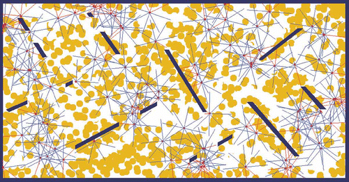
Figure 1. Snapshot from the simulator with 100 agents. Food items are represented as circles. Agents are represented with proximity sensor rays, modelled on the e-puck robot. Communication range is half the range of proximity sensors.

Table 1. Parameters for experiments

Table 2. Parameters for experiments – specific to the ‘energy’ set-up

Figure 2. Experimental results -- the experiment starts with the ‘free-ride’ set-up from generation 0 to generation 75, then it switches to the ‘energy’ set-up until generation 150. Note that artefacts can be explained by the initial set-up conditions. Firstly, generation 0 starts with agents' starting locations drawn from a normal distribution (i.e. all agents are close to one another), which explains the initial slight decrease in the number of active agents in the first generations (i.e. some agents quickly end up in deserted areas). Secondly, generation 75 (i.e. first generation following the switch to the ‘energy’ set-up) considers agents with an initial energy level of 500 units, which happens to be sufficient to enable survival of unfit (i.e. food items harvesting is slower than energy loss), but lucky, genomes for a few generations. (a) Active agents per generation; (b) number of imported genomes per agent; (c) Average evergy balance per agents; and (d) parameter for Gaussion mutation.
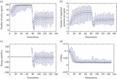
Figure 2. Experimental results -- the experiment starts with the ‘free-ride’ set-up from generation 0 to generation 75, then it switches to the ‘energy’ set-up until generation 150. Note that artefacts can be explained by the initial set-up conditions. Firstly, generation 0 starts with agents' starting locations drawn from a normal distribution (i.e. all agents are close to one another), which explains the initial slight decrease in the number of active agents in the first generations (i.e. some agents quickly end up in deserted areas). Secondly, generation 75 (i.e. first generation following the switch to the ‘energy’ set-up) considers agents with an initial energy level of 500 units, which happens to be sufficient to enable survival of unfit (i.e. food items harvesting is slower than energy loss), but lucky, genomes for a few generations. (a) Active agents per generation; (b) number of imported genomes per agent; (c) Average evergy balance per agents; and (d) parameter for Gaussion mutation.

Figure 3. Experimental results for some (randomly chosen) specific runs. Note the oscillations during the ‘energy’ set-up – these oscillations are smoothed and shadowed in because of the large number of runs considered. (a)–(d) The number of active agents oscillates around the stable solution for mEDEA in this experiment (i.e. a larger population cannot survive in the environment, while a smaller population does not exploit all available resources. Oscillations are due to food regrowing (see text for details)).
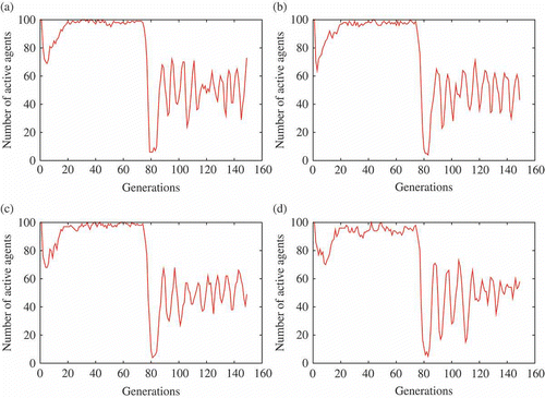
Figure 3. Experimental results for some (randomly chosen) specific runs. Note the oscillations during the ‘energy’ set-up – these oscillations are smoothed and shadowed in Figure 2 because of the large number of runs considered. (a)–(d) The number of active agents oscillates around the stable solution for mEDEA in this experiment (i.e. a larger population cannot survive in the environment, while a smaller population does not exploit all available resources. Oscillations are due to food regrowing (see text for details)).

Figure 4. Genome battles on both set-ups ((a) free-ride set-up ; (b) energy set-up). Average success scores for each generation – both histograms are the results of 1000+ battles (see text for details).

Figure 4. Genome battles on both set-ups ((a) free-ride set-up ; (b) energy set-up). Average success scores for each generation – both histograms are the results of 1000+ battles (see text for details).

Figure 5. Typical examples of agents' behavioural traces in the free-ride set-up. The square symbol shows the agents' starting points. Agents are tested in environments with or without walls (i.e. black bars).
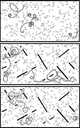
Figure 5. Typical examples of agents' behavioural traces in the free-ride set-up. The square symbol shows the agents' starting points. Agents are tested in environments with or without walls (i.e. black bars).

Figure 6. Typical examples of agents' behavioural traces in the energy set-up. The coloured traces account for the current energy level of the agent. The square symbol shows the agents' starting points. Agents are tested in environments with or without walls.
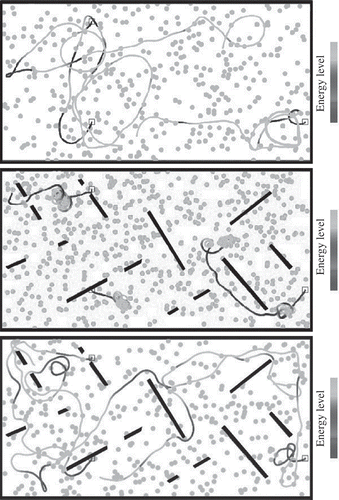
Figure 6. Typical examples of agents' behavioural traces in the energy set-up. The coloured traces account for the current energy level of the agent. The square symbol shows the agents' starting points. Agents are tested in environments with or without walls.

Figure 7. The ‘two-suns’ set-up: a population of agents is dropped into an empty environment where a ‘sun’ is present (the circle on the left of the image). Each agent gets information about its distance and orientation with respect to the sun, but the sun itself gives no direct advantage whatsoever (e.g. no energy). Every 50 generations, the current sun disappears and another sun appears at the opposite end of the arena.
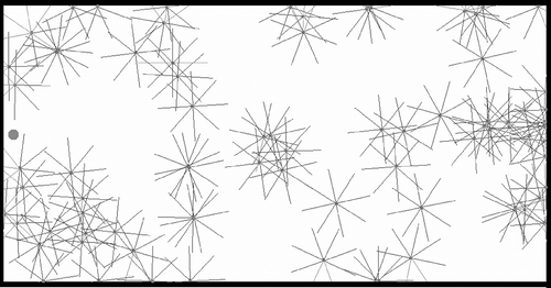
Figure 7. The ‘two-suns’ set-up: a population of agents is dropped into an empty environment where a ‘sun’ is present (the circle on the left of the image). Each agent gets information about its distance and orientation with respect to the sun, but the sun itself gives no direct advantage whatsoever (e.g. no energy). Every 50 generations, the current sun disappears and another sun appears at the opposite end of the arena.

Figure 8. Number of successful runs (out of 24, for each population size) for different values of radio communication length: (a) , (b) ; and (c) . A run is successful whenever at least one agent is still alive at the end of the last generation. In practice, however, successful runs always feature healthy population (i.e. most agents are alive). These graphs illustrate an abrupt phase transition in the parameter space (considering population size and radio communication length) before which agents do not survive (i.e. mating becomes too difficult).
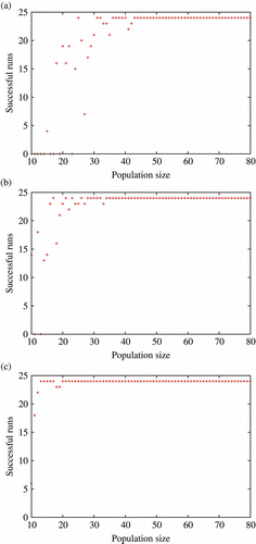
Figure 8. Number of successful runs (out of 24, for each population size) for different values of radio communication length: (a) , (b) ; and (c) . A run is successful whenever at least one agent is still alive at the end of the last generation. In practice, however, successful runs always feature healthy population (i.e. most agents are alive). These graphs illustrate an abrupt phase transition in the parameter space (considering population size and radio communication length) before which agents do not survive (i.e. mating becomes too difficult).

Figure 9. Example of run where the population faces extinction (extracted from one run with , ). This is but one particular example of run leading to extinction and is displayed here for illustration purpose. In this run, the agents were actually able to reach a consensus for some time. However, the relatively low population and medium communication range created a context within which a series of unsuccessful mutation (around generation 120) could not be recovered from and quickly lead to complete extinction. (a) Agents' orientation and (b) agents' distance with respect to the centre of the environment (heat map).
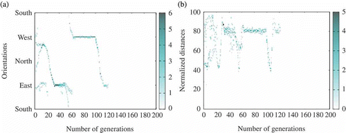
Figure 9. Example of run where the population faces extinction (extracted from one run with , ). This is but one particular example of run leading to extinction and is displayed here for illustration purpose. In this run, the agents were actually able to reach a consensus for some time. However, the relatively low population and medium communication range created a context within which a series of unsuccessful mutation (around generation 120) could not be recovered from and quickly lead to complete extinction. (a) Agents' orientation and (b) agents' distance with respect to the centre of the environment (heat map).

Figure 10. Tracking agents' orientation and distance to the centre of the environment for different population sizes and experimental set-ups, in the final iteration of the experiment (i.e. snapshot of the last moment of the experiment). Three different communication radii are considered. Graphs in the left column show the orientations of agents with regard to the centre of the environment. Graphs in the right column show agents' distances to the centre of the environment. The three pairs of graphs correspond, respectively, to experiments where the communication radius is set to 16 (first row), 32 (second row) and 64 (third row). For each graph, darker regions in the graphs indicate the most commonly observed orientation/distance w.r.t. the centre at the end of experiment (y-axis) for each population size parameter (x-axis) with a given communication radius value (table rows) -- this representation scheme is commonly known as a heat map. Each row is the result of aggregation of 1704 independent runs.
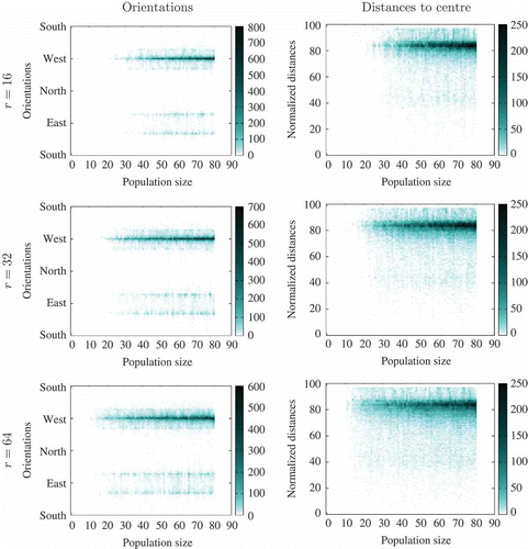
Figure 10. Tracking agents' orientation and distance to the centre of the environment for different population sizes and experimental set-ups, in the final iteration of the experiment (i.e. snapshot of the last moment of the experiment). Three different communication radii are considered. Graphs in the left column show the orientations of agents with regard to the centre of the environment. Graphs in the right column show agents' distances to the centre of the environment. The three pairs of graphs correspond, respectively, to experiments where the communication radius is set to 16 (first row), 32 (second row) and 64 (third row). For each graph, darker regions in the graphs indicate the most commonly observed orientation/distance w.r.t. the centre at the end of experiment (y-axis) for each population size parameter (x-axis) with a given communication radius value (table rows) -- this representation scheme is commonly known as a heat map. Each row is the result of aggregation of 1704 independent runs.

Table 3. Various types of consensus

Figure 11. Example of consensus towards the sun (extracted from one run with , ). Distances vary between 0 (agent in the centre of the environment) and 100 (agent in a corner). (a) Agents' orientation and (b) distance with respect to the centre of the environment (heat map).
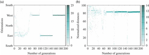
Figure 11. Example of consensus towards the sun (extracted from one run with , ). Distances vary between 0 (agent in the centre of the environment) and 100 (agent in a corner). (a) Agents' orientation and (b) distance with respect to the centre of the environment (heat map).
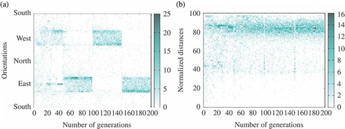
Figure 12. Example of consensus towards the side opposite to the sun (extracted from one run with , ). (a) Agents' orientation and (b) distance with respect to the centre of the environment (heat map).
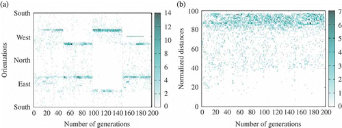
Figure 12. Example of consensus towards the side opposite to the sun (extracted from one run with , ). (a) Agents' orientation and (b) distance with respect to the centre of the environment (heat map).

Figure 13. Example of several simultaneous consensus during one run (extracted from one run with , ). (a) Agents' orientation and (b) distance with respect to the centre of the environment (heat map).

Figure 13. Example of several simultaneous consensus during one run (extracted from one run with , ). (a) Agents' orientation and (b) distance with respect to the centre of the environment (heat map).

Figure 14. Example of a run where agents ignore the sun, except at the very end (extracted from one run with , ). (a) Agents' orientation and (b) agents' distance with respect to the centre of the environment (heat map).
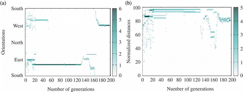
Figure 14. Example of a run where agents ignore the sun, except at the very end (extracted from one run with , ). (a) Agents' orientation and (b) agents' distance with respect to the centre of the environment (heat map).

Figure 15. (a) E-puck Linux extension board with USB WiFi card (casing removed). (b) An e-puck with Linux board fitted in-between the e-puck motherboard (lower) and the e-puck speaker board (upper). Also note the yellow ‘hat’ which here serves three different functions: (1) it provides a matrix of pins for the reflective spheres which allow the tracking system to identify and track each robot and (2) it provides a mounting for the USB WiFi card which slots in horizontally (the wires connecting to the WiFi card are above the USB connector). (c) Experimental swarm robotics arena with 10 Linux extended e-pucks.
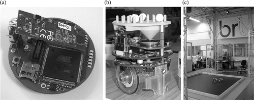
Figure 15. (a) E-puck Linux extension board with USB WiFi card (casing removed). (b) An e-puck with Linux board fitted in-between the e-puck motherboard (lower) and the e-puck speaker board (upper). Also note the yellow ‘hat’ which here serves three different functions: (1) it provides a matrix of pins for the reflective spheres which allow the tracking system to identify and track each robot and (2) it provides a mounting for the USB WiFi card which slots in horizontally (the wires connecting to the WiFi card are above the USB connector). (c) Experimental swarm robotics arena with 10 Linux extended e-pucks.

Figure 16. Experimental infrastructure for swarm robotics research based on the Linux extended e-puck. The swarm lab server provides a data-logging capability that combines and time stamps position-tracking data collected by the ViconTM system with robot status and sensor data from the e-pucks via WiFi, into a log file for post-analysis of experimental runs.

Figure 16. Experimental infrastructure for swarm robotics research based on the Linux extended e-puck. The swarm lab server provides a data-logging capability that combines and time stamps position-tracking data collected by the ViconTM system with robot status and sensor data from the e-pucks via WiFi, into a log file for post-analysis of experimental runs.

Figure 17. Illustration from the experiment described in the text. (a) Emergence of consensus to go towards the sun. (b) Impact of changing the sun location, which shows the human changing the sun location, and convergence of the robots to the new location.
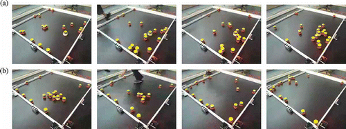
Figure 17. Illustration from the experiment described in the text. (a) Emergence of consensus to go towards the sun. (b) Impact of changing the sun location, which shows the human changing the sun location, and convergence of the robots to the new location.

Figure 18. Number of active robots during the course of a selected experiment. Small bars correspond to one of the robots restarting. The high bar corresponds to the sun location changing event.
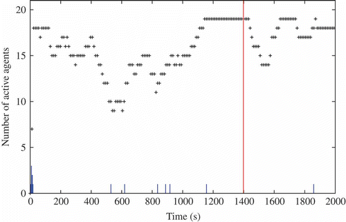
Figure 18. Number of active robots during the course of a selected experiment. Small bars correspond to one of the robots restarting. The high bar corresponds to the sun location changing event.

Figure 19. Distance of the robots to the sun at every time step during the course of a selected experiment. Darker regions imply more robots are located at this particular distance from the sun. The high bar corresponds to the sun location changing event.
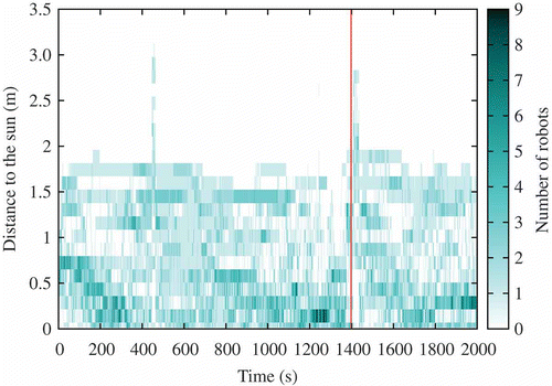
Figure 19. Distance of the robots to the sun at every time step during the course of a selected experiment. Darker regions imply more robots are located at this particular distance from the sun. The high bar corresponds to the sun location changing event.

Figure 20. Tracking the values for each robot at each generation of genes related to the sun orientation: NN weights connecting the sun's orientation to agent rotational speed (sun-orientation gene) and agent translation speed (sun-distance gene). The high bar corresponds to sun location changing event.
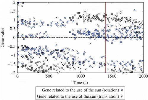
Figure 20. Tracking the values for each robot at each generation of genes related to the sun orientation: NN weights connecting the sun's orientation to agent rotational speed (sun-orientation gene) and agent translation speed (sun-distance gene). The high bar corresponds to sun location changing event.

Reprints and Corporate Permissions

Please note: Selecting permissions does not provide access to the full text of the article, please see our help page How do I view content?

To request a reprint or corporate permissions for this article, please click on the relevant link below:

Academic Permissions

Please note: Selecting permissions does not provide access to the full text of the article, please see our help page How do I view content?

Obtain permissions instantly via Rightslink by clicking on the button below:

If you are unable to obtain permissions via Rightslink, please complete and submit this Permissions form. For more information, please visit our Permissions help page.