Publication Cover
Mathematical and Computer Modelling of Dynamical Systems
Methods, Tools and Applications in Engineering and Related Sciences
Volume 18, 2012 - Issue 3
440
Views
6
CrossRef citations to date
0
Altmetric
Original Articles

Grey-box modelling of a viscose-fibre drying process

, , &
Pages 307-325 | Received 30 Oct 2009, Accepted 20 Jan 2012, Published online: 27 Feb 2012

Figures & data

Figure 1. Scheme of the dryer: the transportation path of the fibre belt and the flow directions of the drying air are indicated as well as the insertion of water and the moisture measurement.

Figure 1. Scheme of the dryer: the transportation path of the fibre belt and the flow directions of the drying air are indicated as well as the insertion of water and the moisture measurement.

Figure 2. Scheme of a plane fibre web element with index i: X moisture content in the fibres, Y humidity of air, m F mass of dry fibres, mA mass of dry air, mass flow of dry fibres, mass flow of dry air, actual mass flow of evaporating water, and h specific enthalpy. Subscript A stands for air, V for vapour, i for element index, and in for the respective input value.
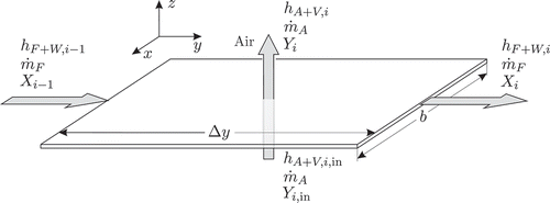
Figure 2. Scheme of a plane fibre web element with index i: X moisture content in the fibres, Y humidity of air, m F mass of dry fibres, mA mass of dry air, mass flow of dry fibres, mass flow of dry air, actual mass flow of evaporating water, and h specific enthalpy. Subscript A stands for air, V for vapour, i for element index, and in for the respective input value.

Figure 3. Interactions between fibre, water, air and vapour in a model element with index i.

Figure 3. Interactions between fibre, water, air and vapour in a model element with index i.

Figure 4. Scheme of the cellulosic fibre molecular structure.

Figure 4. Scheme of the cellulosic fibre molecular structure.

Figure 5. Validation of identified disturbance model. The disturbance is given by a variation in fibre sheet thickness.
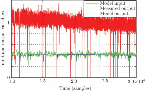
Figure 5. Validation of identified disturbance model. The disturbance is given by a variation in fibre sheet thickness.

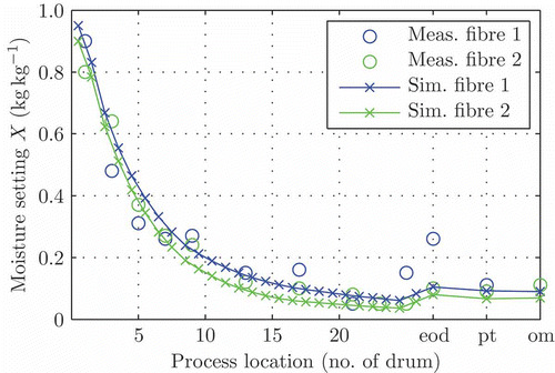
Figure 6. Validation with different fibre types at different operation points.

Figure 6. Validation with different fibre types at different operation points.

Figure 7. Validation with different fibre types at different operation points; the numbers at the axis ‘process location’ are the numbers of the drums, ‘eod’ means ‘end of dryer’ (after the moistener), ‘pt’ means ‘pneumatic transportation’ and ‘om’ stands for ‘online measurement’.
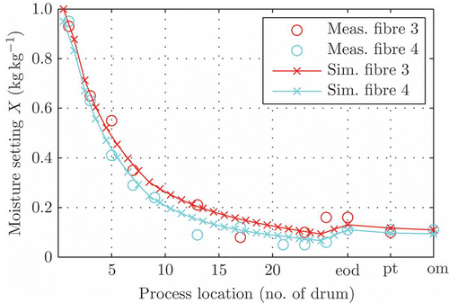
Figure 7. Validation with different fibre types at different operation points; the numbers at the axis ‘process location’ are the numbers of the drums, ‘eod’ means ‘end of dryer’ (after the moistener), ‘pt’ means ‘pneumatic transportation’ and ‘om’ stands for ‘online measurement’.

Figure 8. Simulation of transient behaviour; X 0 is the incoming moisture setting of the fibres, X 1 until X 8 is the moisture setting at each drum. At t = 1500 s X 0 takes a step to X 0 = 0.9, at t = 2500 s the fibrous web becomes thinner and at t = 3500 s temperature of drying air decreases by 5°C at every drum. Moisture settings Xi are normalized.
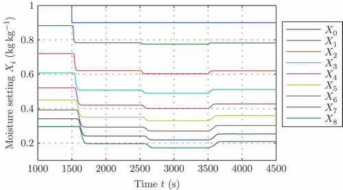
Figure 8. Simulation of transient behaviour; X 0 is the incoming moisture setting of the fibres, X 1 until X 8 is the moisture setting at each drum. At t = 1500 s X 0 takes a step to X 0 = 0.9, at t = 2500 s the fibrous web becomes thinner and at t = 3500 s temperature of drying air decreases by 5°C at every drum. Moisture settings Xi are normalized.

Figure 9. Sensitivity analysis of temperature levels in the dryer; the predryer consists of the drums 1–8, the main dryer of the drums 9–24.
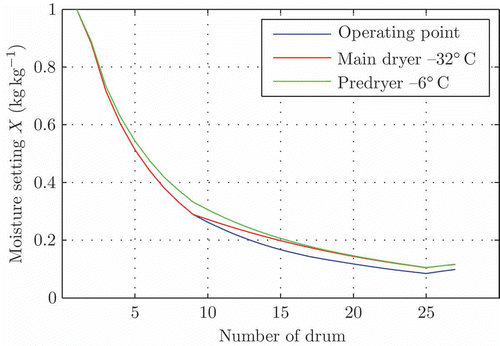
Figure 9. Sensitivity analysis of temperature levels in the dryer; the predryer consists of the drums 1–8, the main dryer of the drums 9–24.

Figure 10. Dynamical Validation: (a) the output signal y with its typical variance is shown; (b) a case with measurable disturbance (fibre sheet thickness) is depicted.
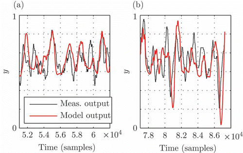
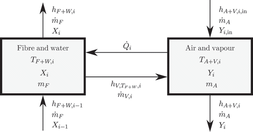
Figure 10. Dynamical Validation: (a) the output signal y with its typical variance is shown; (b) a case with measurable disturbance (fibre sheet thickness) is depicted.
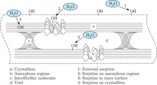
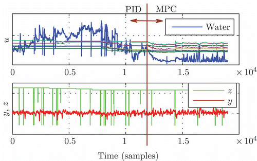
Figure 11. Comparison between PID and MPC strategy. u are the manipulated variables (heating power and water), z is a disturbance variable (fibre sheet thickness) and y is the controlled variable.

Figure 11. Comparison between PID and MPC strategy. u are the manipulated variables (heating power and water), z is a disturbance variable (fibre sheet thickness) and y is the controlled variable.

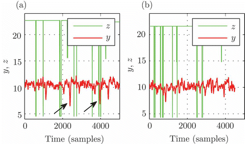
Figure 12. Comparison between PID (a) and MPC (b) strategy: compensation of a measurable disturbance. z is a disturbance variable (fibre sheet thickness) and y the controlled variable (moisture setting). Arrows in the left plot indicate uncompensated disturbances during PID control.

Figure 12. Comparison between PID (a) and MPC (b) strategy: compensation of a measurable disturbance. z is a disturbance variable (fibre sheet thickness) and y the controlled variable (moisture setting). Arrows in the left plot indicate uncompensated disturbances during PID control.

Reprints and Corporate Permissions

Please note: Selecting permissions does not provide access to the full text of the article, please see our help page How do I view content?

To request a reprint or corporate permissions for this article, please click on the relevant link below:

Academic Permissions

Please note: Selecting permissions does not provide access to the full text of the article, please see our help page How do I view content?

Obtain permissions instantly via Rightslink by clicking on the button below:

If you are unable to obtain permissions via Rightslink, please complete and submit this Permissions form. For more information, please visit our Permissions help page.