Predicting high-codimension critical transitions in dynamical systems using active learning

Figures & data

Figure 1. Dynamics for choice of (q, r) exhibiting three steady states.

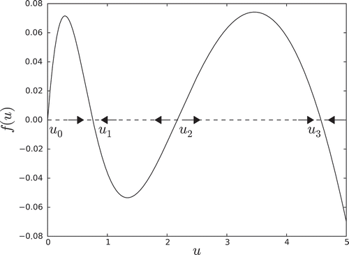
Figure 2. Isolating neighbourhoods for equilibria u₁, u₂, u₃ from Figure 1 as a function of parameter q and a fixed r. The isolating neighbourhood for u₀ is omitted for clarity.

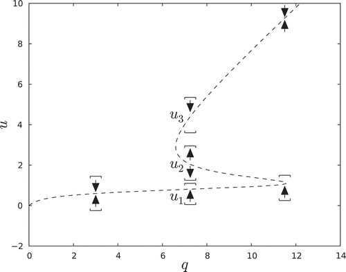
Figure 3. Morse graph for Morse decomposition for M (S_q), q = 7.5, see Figure 2. (u₀ has been included.)

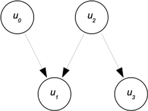
Figure 4. (a) Equilibria states in a general cusp catastrophe model. In the region of the fold, three equilibrium states exist. One equilibrium exists in other regions. The dashed vertical line shows the arrangement of the equilibria in phase space for an arbitrary pair of parameters (q, r) in the cusp region. The repeller and attractors in the Morse graph in Figure 3 correspond to u₁, u₂ and u₃. (b) Parameter space showing the projection of the folded region on the right.

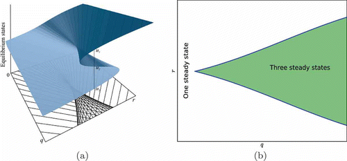
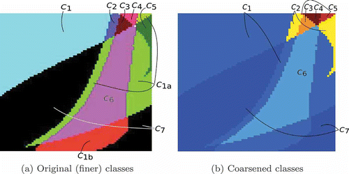
Figure 5. A slice of parameter space at z = 1. (a) Continuation classes from the original paper by Arai et al.; (b) Classes obtained without machine learning algorithms, but using the coarser notion of equivalence. Classes labels, C_*, correspond between (a) and (b) as well as to those in the figures below (colour online).

Table

AlgorithmD
1 M ← m     ▹ Max size of training set
2  uniform random samples from .
▹ Initial training set used to construct
▹ a preliminary triangulation.
3 .
4 Compute  ▹ Delaunay triangulation of the current training set .
5 repeat Q0 ← uniform random sample from
6    Find , such that Q0 ∈ S0
7    if All the vertices of S0 have isomorphic Morse graphs
8    then and .
9  until
10 return

Table

AlgorithmN
1 M ← m     ▹ Max size of training set
2  uniform random samples from
▹ Initial training set used to construct
▹ a preliminary triangulation.
3 repeat Q0 ← uniform random sample from
4     .
5     -nearest neighbors of Q0 in .
6     if majority MG(Q) for not isomorphic
▹ Using specified majority rule
7     then and
8  until
9 return

Figure 6. (a) z slice 1, training set size 10% of , misclassification of 244 points, or 3.8125% classification error; (b) z slice 9, training set size 20% of , misclassification of 79 points, or 1.234% classification error. As in Figure 5, classes that correspond across the slices are labelled the same. Notice that in (b) class C′₂ is a newly detected class, while the dynamics detected in classes C₂ and C₃ do not show up in the z = 9 slice of parameter space.

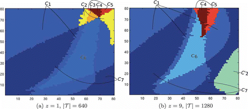
Figure 7. Delaunay triangulation of generated using AlgorithmD; z = 9, .

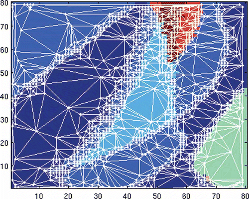
Table 1. Results for compilation of 2D z slices for AlgorithmD, AlgorithmN and Uniform Sampling.

Training set %	AlgorithmD	AlgorithmN	Uniform
10%	4.5	4.9	7.13
20%	1.1	2.78	4.98

Figure 8. Plot of training set for AlgorithmN on z = 1, , misclassification of 123 grid elements, or 1.92% of ; the shade of a training set element depends upon when it was selected in the process of constructing . Classes correspond to those in Figures 5 and 6.

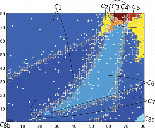
Table 2. Results for 3D Variants of AlgorithmN and Uniform Sampling.

Training set %	AlgorithmN	Uniform
10%	5.74	7.46
20%	3.19	5.86