Dimension reduction for second-order systems by general orthogonal polynomials

Figures & data

Table 1. Differential recurrence coefficients for classical orthogonal polynomials.

Orthogonal polynomial	${\alpha }_i$	${\beta }_i$	${\gamma }_i$
Chebyshev-1	$\frac{1}{2i+2}$	0	$-\frac{1}{2i-2}$
Chebyshev-2	$\frac{1}{2i+2}$	0	$-\frac{1}{2i+2}$
Legendre	$\frac{1}{2i+1}$	0	$-\frac{1}{2i+1}$
Laguerre	$-\frac{1}{i+1}$	1	0
Hermite	$-\frac{1}{2i+2}$	0	0
Jacobi $(\alpha >-1,\beta >-1)$	$\frac{2(\alpha +\beta +i+1)}{(\alpha +\beta +2i+2)(\alpha +\beta +2i+1)}$	$\frac{2(\alpha -\beta )}{(\alpha +\beta +2i)(\alpha +\beta +2i+2)}$	$\frac{-2(\alpha +i)(\beta +i)}{(\alpha +\beta +2i)(\alpha +\beta +i)}$

Figure 1. Transient responses (a) and relative errors (b) of the reduced models obtained by Algorithm 1, the BTR method and the Arnoldi method in Example 1.

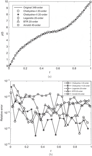
Figure 2. Transient responses (a) and relative errors (b) of the reduced models obtained by Algorithm 2, the SOBT method and the SOAR method in Example 1.

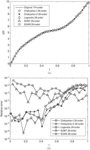
Table 2. Computational times of obtaining reduced models for Example 1.

	Chebyshev-1	Chebyshev-2	Legendre	SOBT	SOAR
Time (s)	4.10	4.08	4.09	1.28	0.075

Figure 3. Transient responses (a) and relative errors (b) of the output $y_3(t)$ of the reduced models obtained by Algorithm 2, the SOBT method and the SOAR method in Example 2.

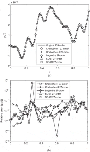
Table 3. Computational times of obtaining reduced models for Example 2.

	Chebyshev-1	Chebyshev-2	Legendre	SOBT	SOAR
Time (s)	0.062	0.060	0.068	0.37	0.020

Figure 4. Transient responses (a) and relative errors (b) of the reduced models obtained by Algorithm 2, the SOBT method and the SOAR method in Example 3.

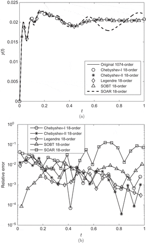
Table 4. Computational times of obtaining reduced models for Example 3.

	Chebyshev-1	Chebyshev-2	Legendre	SOBT	SOAR
Time (s)	20.61	16.37	16.08	20.20	1.09