Publication Cover
Mathematical and Computer Modelling of Dynamical Systems
Methods, Tools and Applications in Engineering and Related Sciences
Volume 22, 2016 - Issue 2
274
Views
7
CrossRef citations to date
0
Altmetric
Original Articles

On unifying concepts for trajectory-based slow invariant attracting manifold computation in kinetic multiscale models

&
Pages 87-112 | Received 17 Oct 2014, Accepted 08 Jan 2016, Published online: 02 Mar 2016

Figures & data

Figure 1. Solutions z1(tf = 0; t0) of the boundary value formulation (27) applied to the linear model (1) with γ = 0.2 visualized by the rhombi in comparison with the analytical error (33) (dashed line) as a function of t0.
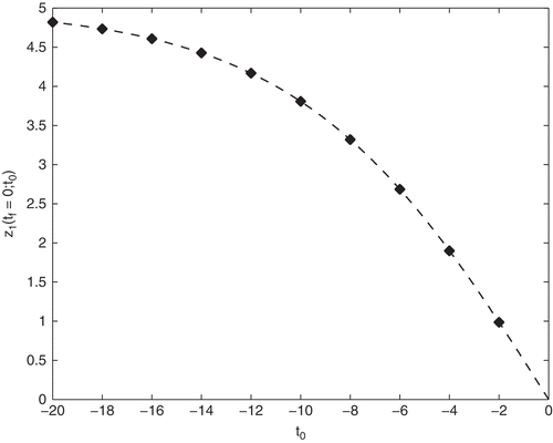
Figure 1. Solutions z1(tf = 0; t0) of the boundary value formulation (27) applied to the linear model (1) with γ = 0.2 visualized by the rhombi in comparison with the analytical error (33) (dashed line) as a function of t0.
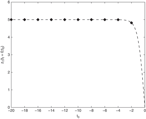
Figure 2. Solutions z1(tf = 0; t0) of the boundary value problem (27) applied to the linear model (1) with γ = 2.0 visualized by the rhombi in comparison with the analytical error (33) (dashed line) as a function of t0.

Figure 2. Solutions z1(tf = 0; t0) of the boundary value problem (27) applied to the linear model (1) with γ = 2.0 visualized by the rhombi in comparison with the analytical error (33) (dashed line) as a function of t0.

Figure 3. Solutions z2(tf = 0; Z0) of the boundary value formulation (27) applied to the Davis–Skodje test problem (2) with γ = 1.2 visualized by the rhombi in comparison with the analytical error (39) (dashed line) as a function of t0.
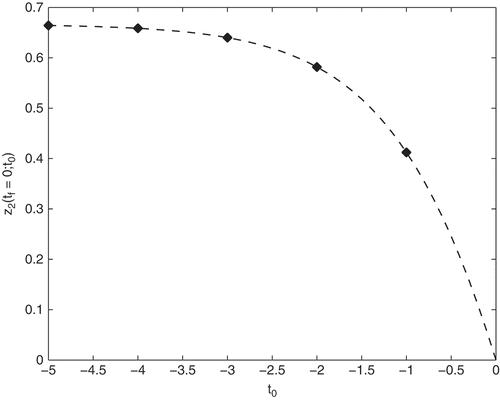
Figure 3. Solutions z2(tf = 0; Z0) of the boundary value formulation (27) applied to the Davis–Skodje test problem (2) with γ = 1.2 visualized by the rhombi in comparison with the analytical error (39) (dashed line) as a function of t0.
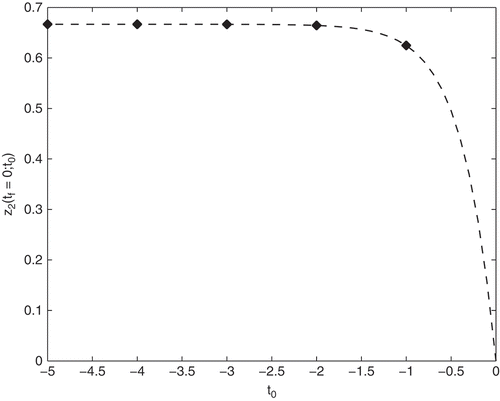
Figure 4. Solutions z2(tf = 0; t0) of the boundary value formulation (27) applied to the Davis–Skodje test problem (2) with γ = 3.0 visualized by the rhombi in comparison with the analytical error (39) (dashed line) as a function of t0.

Figure 4. Solutions z2(tf = 0; t0) of the boundary value formulation (27) applied to the Davis–Skodje test problem (2) with γ = 3.0 visualized by the rhombi in comparison with the analytical error (39) (dashed line) as a function of t0.

Figure 5. POIs (crosses) resulting from optimization problem (49) applied to a simplified six species mechanism (see [Citation45]) with z(H2O) as RPV fixed at 80 different values between zjtf=104 and zjtf=4.0. As can be seen, the POIs form an invariant manifold attracting several reaction trajectories (dashed curves) starting from arbitrarily chosen initial values.

Figure 5. POIs (crosses) resulting from optimization problem (49) applied to a simplified six species mechanism (see [Citation45]) with z(H2O) as RPV fixed at 80 different values between zjtf=10−4 and zjtf=4.0. As can be seen, the POIs form an invariant manifold attracting several reaction trajectories (dashed curves) starting from arbitrarily chosen initial values.

Figure 6. Visual demonstration why a reverse mode formulation works more accurately than the corresponding local method. A polyhedron restricts the feasible area with the consequence that t0 can only be chosen as small as possible within the feasibility constraints.
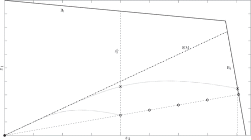
Figure 6. Visual demonstration why a reverse mode formulation works more accurately than the corresponding local method. A polyhedron restricts the feasible area with the consequence that t0 can only be chosen as small as possible within the feasibility constraints.

Figure 7. The black dots represent the equilibrium point, the solid curves the SIM and the dashed curves are solution trajectories concerning the underlying model equations. (a) Linear model. (b) Davis–Skodje model.
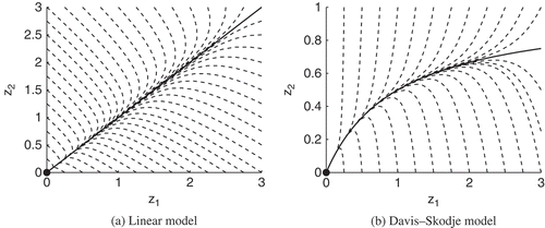
Figure 7. The black dots represent the equilibrium point, the solid curves the SIM and the dashed curves are solution trajectories concerning the underlying model equations. (a) Linear model. (b) Davis–Skodje model.

Reprints and Corporate Permissions

Please note: Selecting permissions does not provide access to the full text of the article, please see our help page How do I view content?

To request a reprint or corporate permissions for this article, please click on the relevant link below:

Academic Permissions

Please note: Selecting permissions does not provide access to the full text of the article, please see our help page How do I view content?

Obtain permissions instantly via Rightslink by clicking on the button below:

If you are unable to obtain permissions via Rightslink, please complete and submit this Permissions form. For more information, please visit our Permissions help page.