A POD–EIM reduced two-scale model for precipitation in porous media

Figures & data

Figure 1. The considered initial configuration ℐ of the three substances in the microscopic pore-space μ, where $Y=\mathcal{G}\cup {\mathrm{\Gamma }}_{\mathcal{G}}\cup \mathcal{P}$. The grain μ is located in the centre of Y and the pore-space μ is occupied by the two immiscible and incompressible fluids P₁ (water) and P₂ (oil) as well as the precipitate P₂. The spherical perforated precipitate P₃ is attached to the boundary Г_μ of the grain μ, the spherical fluid P₂ domain is located in the corners of the microscopic domain Y and the fluid P₁ occupies the remainder.

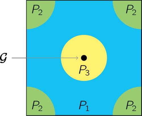
Table 1. The varying parameters of the three settings S₁, S₂ and S₃, which are explained in Section 4.1 and Figure 2. The function u_(t) = a:b increases linearly from a to b with the time-steps in the course of a simulation. For i = 1,2 an initial precipitate’s radius $r_0(i)$ results in a precipitate’s initial portion of ${\overline{{\varphi }_3}}^{\mathcal{P}}(i)$ on the overall pore-space’s volume, analogously the water’s initial portion is ${\overline{{\varphi }_1}}^{\mathcal{P}}(i)$, and the oil’s initial portion is ${\overline{{\varphi }_2}}^{\mathcal{P}}(i)=0.07$ due to a radius ${\tilde{r}}_0(i)=30h_{\mathrm{\ell }}$.

Setting	T	H	$u_0$	$u_{\mathrm{\perp }}(t)$	$r_0$	${\overline{{\varphi }_1}}^{\mathcal{P}}$	${\overline{{\varphi }_3}}^{\mathcal{P}}$
S1	5	{50,25}	0.4	0.6:0.9	$\{30h_{\mathrm{\ell }},70h_{\mathrm{\ell }}\}$	$\{0.86,0.54\}$	$\{0.07,0.39\}$
S2	2.5	{25,25}	0.5	0.5:0.8	$\{70h_{\mathrm{\ell }},30h_{\mathrm{\ell }}\}$	$\{0.54,0.86\}$	$\{0.39,0.07\}$
S3	2.5	{25,25}	0.5	0.5:0.75	$\{68h_{\mathrm{\ell }},35h_{\mathrm{\ell }}\}$	$\{0.56,0.83\}$	$\{0.37,0.10\}$

Figure 2. The initial phase configurations in the microscopic pore-space ${\mathcal{P}}_{h_{\mathrm{\ell }}}$ in the two subdomains ${\mathrm{\Omega }}_{h_g}^{(1)}$ and ${\mathrm{\Omega }}_{h_g}^{(2)}$ of the macroscopic domain ${\mathrm{\Omega }}_{h_g}$. The black points in the very centre of ${\mathcal{P}}_{h_{\mathrm{\ell }}}$ in (b) and (c) represent the small spherical grains ${\mathcal{G}}_{h_{\mathrm{\ell }}}$. Each grain is surrounded by a precipitate $P_3$ (yellow). For $i=1,2$, $r_{0,i}$ defines the initial radius of the precipitates in the subdomain ${\mathrm{\Omega }}_{h_g}^{(i)}$. Each precipitate is surrounded by water (blue) and a spherical oil phase $P_2$ (green) is located in the corners of ${\mathcal{P}}_{h_{\mathrm{\ell }}}$. The coloured subdomains P_i are characterized by ${\varphi }_i\ge \frac{1}{2}$ for $i\in I$. Full colour available online.

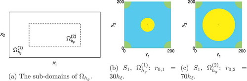
Figure 3. The nodes in the subset ${\mathrm{\Omega }}_{h_g}^{\star }$ of the macroscopic grid ${\mathrm{\Omega }}_{h_g}$: nodes of ${\mathrm{\Omega }}_{h_g}^{\star }\cap {\mathrm{\Omega }}_{h_g}^{(1)}$ are indicated in red, and in blue those of ${\mathrm{\Omega }}_{h_g}^{\star }\cap {\mathrm{\Omega }}_{h_g}^{(2)}$. Full colour available online.

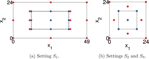
Figure 4. High-dimensional solution of setting $S_1$ at the end of the time-interval for $T=5$.

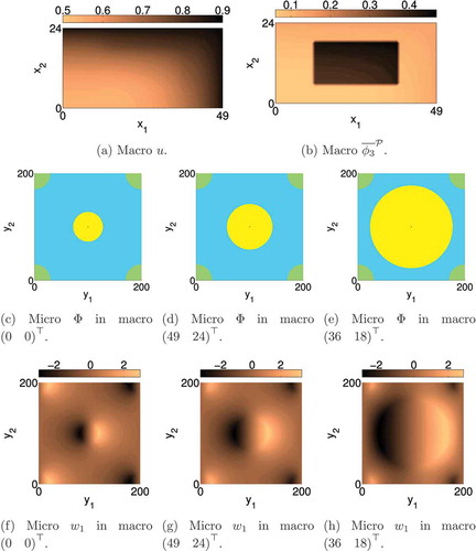
Figure 5. High-dimensional solution of the setting $S_1$: the evolution of the precipitates’ volume portion on the pore-space in the macroscopic nodes $(00{)}^{\mathrm{T}}$ (red dashed), $(126{)}^{\mathrm{T}}$ (blue dotted), $(3618{)}^{\mathrm{T}}$ (black) and $(4924{)}^{\mathrm{T}}$ (cyan). In ${\mathrm{\Omega }}_{h_g}^{(1)}$ the node $(00{)}^{\mathrm{T}}$ (and respectively, $(4924{)}^{\mathrm{T}}$) is host of the precipitate with the minimum (maximum) volume portion throughout the time-interval. The same relation holds in ${\mathrm{\Omega }}_{h_g}^{(2)}$ for $(126{)}^{\mathrm{T}}$ (minimum) and $(3618{)}^{\mathrm{T}}$ (maximum). Full colour available online.

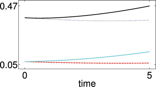
Table 2. Results for setting $S_1$: the column entitled by ‘speed-up’ presents the rough speed-up of the approximations’ computation time in comparison to the high-dimensional solution of $S_1$ in 57 h (as for the high-dimensional solution $27$ processors of type Intel(R) Xeon(R) CPU [email protected] GHz were used), and the columns entitled by $\parallel \mathrm{\Delta }u{\parallel }_Q$, $\parallel \mathrm{\Delta }{K}_{\mathrm{c}\mathrm{o}\mathrm{r}}{\parallel }_Q$, $\parallel \mathrm{\Delta }\mathrm{\Phi }{\parallel }_{Q^{\star }}$ and $\parallel \mathrm{\Delta }({\varphi }_1^{\delta }{w}_1){\parallel }_{Q^{\star }}$ present the approximations’ accuracy. The line entitled by ${\hspace{0.17em}}^{\star }{w}_1=0^{\star }$ presents the results of a high-dimensional approximation with prescribed $w_1=0$ resulting in $K_{\mathrm{c}\mathrm{o}\mathrm{r}}=0$ and ${\varphi }_1^{\delta }{w}_1=0$.

Model	${\epsilon }_{\mathrm{P}\mathrm{O}\mathrm{D}}$	Speed-up	$\parallel \mathrm{\Delta }u{\parallel }_Q$	$\parallel \mathrm{\Delta }{K}_{\mathrm{c}\mathrm{o}\mathrm{r}}{\parallel }_Q$	$\parallel \mathrm{\Delta }\mathrm{\Phi }{\parallel }_{Q^{\star }}$	$\parallel \mathrm{\Delta }({\varphi }_1^{\delta }{w}_1){\parallel }_{Q^{\star }}$
${\hspace{0.17em}}^{\star }{w}_1=0^{\star }$	–	$211$	$3.84e-02$	$1.71e-01$	$5.06e-01$	$2.52e+00$
$R_2$	$1e-02$	$201$	$3.52e-05$	$2.58e-03$	$3.17e-04$	$1.06e-01$
$R_4$	$1e-04$	$200$	$1.57e-05$	$2.58e-03$	$1.95e-04$	$1.06e-01$
$R_6$	$1e-06$	$194$	$5.83e-06$	$7.62e-04$	$1.83e-05$	$1.89e-02$
$R_8$	$1e-08$	$190$	$2.29e-06$	$4.37e-04$	$5.22e-06$	$6.52e-03$
$R_{10}$	$1e-10$	$174$	$4.43e-08$	$1.16e-05$	$3.47e-08$	$5.00e-04$
$R_{12}$	$1e-12$	$149$	$6.49e-09$	$1.45e-06$	$6.63e-09$	$7.39e-05$

Table 3. Results for setting $S_1$: the columns entitled by $N_w$, $|Y_M|$ and $|Y_M^{\ast }|$ present the average sizes of the $100$ basis sets of a reduced model, and the column entitled by ‘reduction time’ presents the time that one processor of type Intel(R) Xeon(R) CPU [email protected] GHz needs to construct the reduced models from the pre-computed snapshots of the high-dimensional solution of $S_1$. In particular, this time is not the full offline time, as it does not include the 57-h for the snapshots computation.

Model	${\epsilon }_{\mathrm{P}\mathrm{O}\mathrm{D}}$	$N_w$	$|Y_M|$	$|Y_M^{\ast }|$	$\sim$Reduction time (h)
$R_2$	$1e-02$	$1.01$	$50.91$	$197.36$	$1.5$hours
$R_4$	$1e-04$	$1.46$	$51.36$	$198.52$	$1.5$hours
$R_6$	$1e-06$	$3.61$	$53.47$	$204.95$	$1.5$hours
$R_8$	$1e-08$	$8.38$	$58.17$	$219.31$	$1.7$hours
$R_{10}$	$1e-10$	$21.75$	$71.11$	$256.47$	$2.1$hours
$R_{12}$	$1e-12$	$51.04$	$95.81$	$318.64$	$3.5$hours

Figure 6. Results for the setting $S_1$ and the low-dimensional solution $R_{10}$ with ${ϵ}_{POD}=1e-10$: (a) presents the evolution of the precipitates’ volumes ${\overline{{\varphi }_3}}^{\mathcal{P}}$ and (b) the utilized basis sets in the course of the simulation in the macroscopic nodes $(00{)}^{\mathrm{T}}$ (red dashed), $(126{)}^{\mathrm{T}}$ (blue dotted), $(3618{)}^{\mathrm{T}}$ (black) and $(4924{)}^{\mathrm{T}}$ (cyan). Full colour available online.

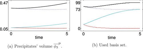
Figure 7. Results for the setting $S_1$ and the low-dimensional solution $R_{10}$: (a) depicts the minimum (black) and maximum (cyan) of the volume interval for the precipitates for the $100$ basis sets that are used in the online phase to determine the proper basis set in order to approximate the reduced solution of $w_1$, where the minimum is $-\mathrm{\infty }$ for basis set $0$ and the maximum is $\mathrm{\infty }$ for basis set $99$; (b) shows the number of POD modes (cyan) and the number of magic points (black) of the basis sets and (c) depicts exemplary for the basis set $73$ for the increasing number of modes the decay of ${log}_{10}$ of the eigenvalues of the correlation operator in the construction of the POD basis (cyan) and for the increasing number of magic points the error decay of the EI (black). Full colour available online.

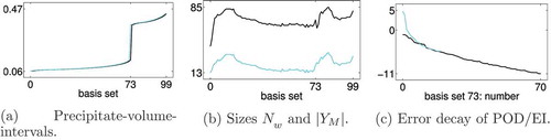
Figure 8. Results for setting $S_1$ and the low-dimensional solution $R_{10}$, which consists of $100$ basis sets: (a), (b) and (c) illustrates the distribution of the magic points in the basis sets $0$, $73$ and $99$, where the inner circle marks the smallest and the outer one the largest subdomain supporting the precipitate in the snapshots, and the four quarters of a circle indicate the almost unchanged oil phase; (d), (e) and (f) depict the dominant POD mode for $w_1$ for the corresponding basis sets.

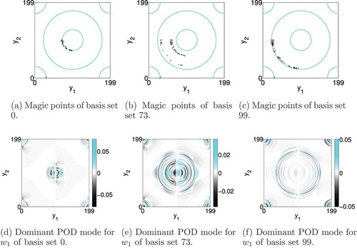
Figure 9. High-dimensional solutions of the settings $S_2$ and $S_3$ in the end of the time-interval at $T=2.5$.

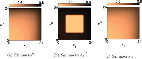
Table 4. Setting S₂: the approximations’ accuracy.

Model	${ϵ}_{POD}$	$\parallel \mathrm{\Delta }u{\parallel }_Q$	$\parallel \mathrm{\Delta }{K}_{11}{\parallel }_Q$	$\parallel \mathrm{\Delta }\mathrm{\Phi }{\parallel }_{Q^{\star }}$	$\parallel \mathrm{\Delta }({\varphi }_1^{\delta }{w}_1){\parallel }_{Q^{\star }}$
*w1 = 0*	–	3.12e − 02	1.71e − 01	1.61e − 01	2.34e + 00
R6	1e − 06	2.23e − 05	3.26e − 04	1.31e − 04	1.93e − 02
R8	1e − 08	7.22e − 06	1.00e − 04	3.40e − 05	1.15e − 02
R10	1e − 10	2.04e − 06	1.32e − 05	1.36e − 06	1.21e − 03
R12	1e − 12	2.21e − 06	1.24e − 05	3.06e − 06	4.13e − 04

Table 5. Setting S₃: the approximations’ accuracy.

Model	${ϵ}_{POD}$	$\parallel \mathrm{\Delta }u{\parallel }_Q$	$\parallel \mathrm{\Delta }{K}_{11}{\parallel }_Q$	$\parallel \mathrm{\Delta }\mathrm{\Phi }{\parallel }_{Q^{\star }}$	$\parallel \mathrm{\Delta }({\varphi }_1^{\delta }{w}_1){\parallel }_{Q^{\star }}$
*w1 = 0*	–	2.46e − 02	1.71e − 01	1.68e − 01	2.42e − 00
R6	1e − 06	2.89e − 05	9.65e − 04	1.23e − 04	2.10e − 02
R8	1e − 08	1.04e − 05	4.29e – 04	9.69e − 05	1.80e − 02
R10	1e − 10	2.36e − 05	1.16e − 03	1.45e − 04	2.63e − 02
R12	1e − 12	2.70e − 05	1.22e − 03	1.44e − 04	2.25e − 02